Densities and Distributions

One of the most natural ways to summarize the lifetimes is bucket the failure times, and then state the proportion of failures in each bucket. Let’s make a plot using that strategy.

data %>% ggplot(aes(lifetime)) + geom_histogram(bins=30)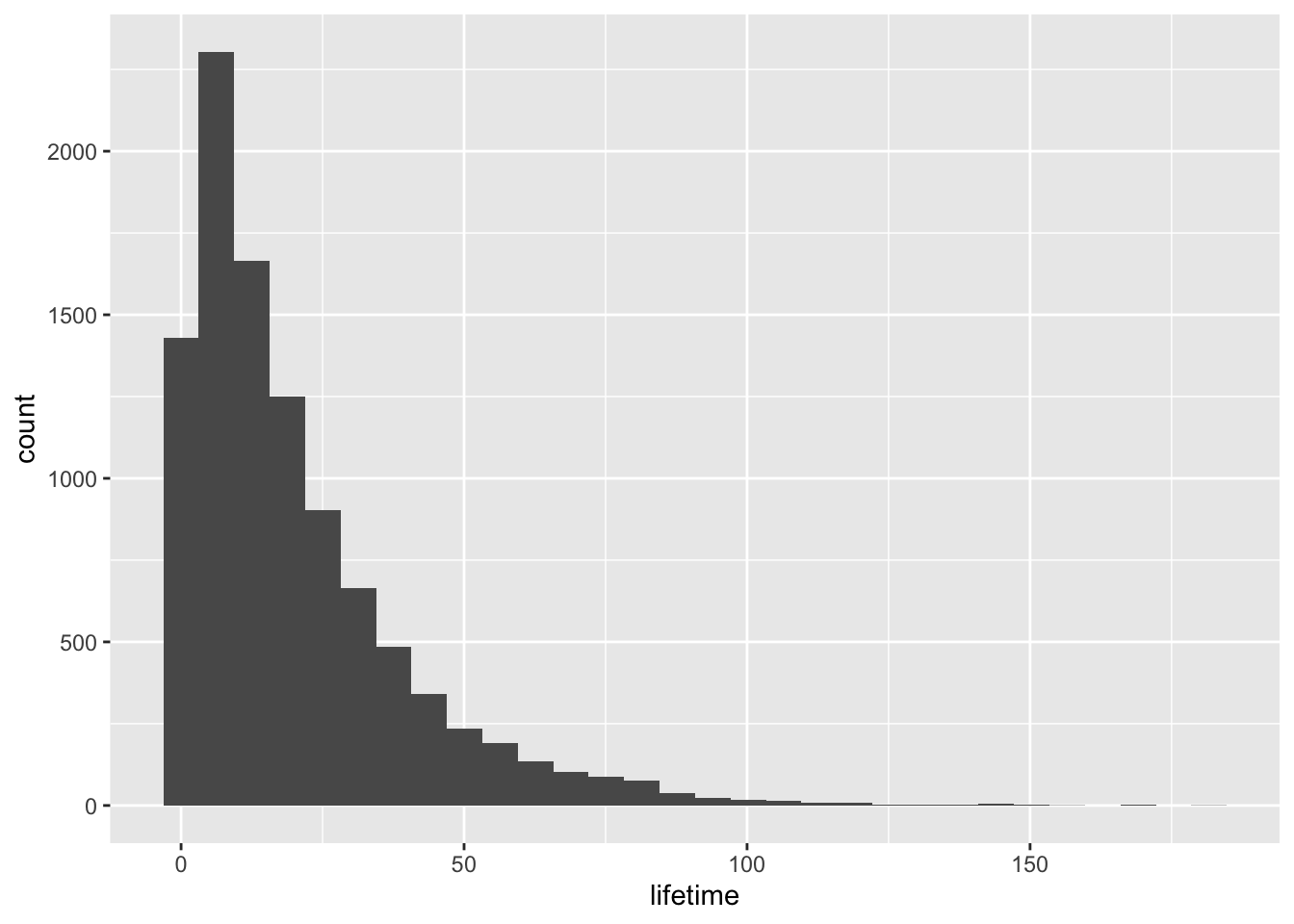

There is one difficulty with this bucketing approach though. We need to pick some arbitrary width for the buckets. If we pick days, for example, then a customer who needs more precision will ask why we didn’t pick hours, and so on. Instead, we can use some cleverness to describe the rate of failure at each instant in time. Then a customer who desires data at any particular granularity can sum over a window of interest to get a probability of failures in that window. We recognize this as our friend the probability density function (PDF) and call it \(f(t)\).

If we could come up with such a function, call it \(f(t)\), and then our customer could calculate the probability of failure between any two times \(t_1\) and \(t_2\). Formally,

\[ P(t_1 \leq T \leq t_2) = \int_{t_1}^{t_2} f(t)dt \]

Another way to describe failure times is with the cumulative distribution function. The cumulative distribution function is simply the proportion of failures up to any time t. \[ F(t) = P(T \leq t) \]

We can plot the distribution function of our data by plotting the proportion of failures up to any time point t.

# Sort the data with the shortest lifetime first.
data <- data %>% arrange(lifetime)
# Count up the number of component that failed before each time point.
data <- data %>% mutate(n_failures = row_number(), proportion_failed=n_failures / n())
head(data)

##   lifetime n_failures proportion_failed
## 1  0.00676          1             1e-04
## 2  0.01017          2             2e-04
## 3  0.01219          3             3e-04
## 4  0.01544          4             4e-04
## 5  0.01623          5             5e-04
## 6  0.01652          6             6e-04

# Plot.
data %>% ggplot(aes(lifetime, proportion_failed)) + geom_line() + ggtitle("Empirical Cumulative Distribution of Lifetimes")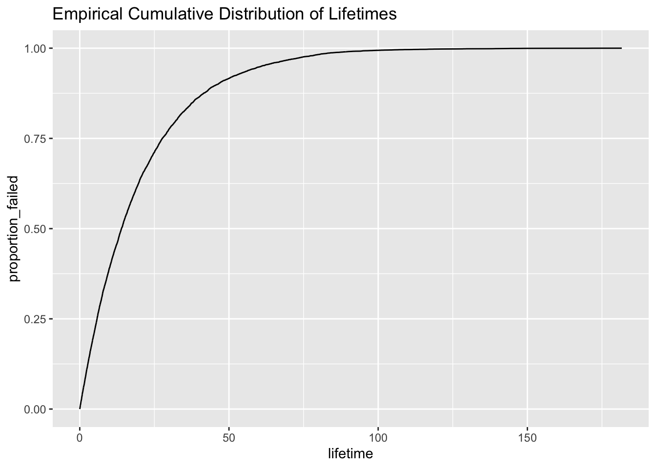

The CDF and PDF have a very simple relationship. Since our PDF gives the rate of failure at each instant in time, the probability of failure from time 0 up to some time t is simply the sum of the PDF multiplied by the width of the interval from 0 up to t. Since our intervals are tiny, integration is required:

\[ F(t) = P(T \leq t) = \int_{0}^{t} f(t)dt \]

Survivor and Hazard

In the case of survival analysis, working with densities and distributions become cumbersome. Instead, statisticians defined two new functions, the survivor and hazard, which are easier to work with. They both have a simple relationship to the distribution and density functions.

The survivor function, S(t), is defined as the probability that a person will survive past time t. That is to say, the survivor function is one minus the distribution function. \[ S(t) = P(T \gt t) = 1 - P(T \leq t) = 1 - F(t) \]

The hazard function, h(t), is the rate at which events occur at time t given that they have survived up to at least time t.

\[ h(t) := \lim_{\delta \to 0}\frac{P(t \leq T \lt t + \delta | T \geq t )}{\delta} \]

This is pretty unintuitive, so let’s unpack how we got to this definition. Going back to our microchips example, we are interested in the proportion of chips that fail within a unit of time. Wouldn’t it be nice to have a function that, given a time in days, t, gives back the proportions of parts that will fail per day?

Say we wanted to find this rate of failure on days 20 and 21. Intuitively, we would look for all chips that failed after day 20, and then count the units that failed between days 20 and 22. We divide these two numbers to get a proportion and then divide by 2 to get the proportion of failures per day. This will be a good approximation of the true failure rate around day 20 if the number of chips we observe, N, is large enough.

\[ \frac{P(20 \leq T \lt 22 | T \geq 20)}{22 - 20} \approx \frac{n_{failed\ betwen\ 20\ and\ 22}}{2} \]

If we repeat this for all even days, then we will have a function telling us how the rate of failure changes over time. For electronic components, we expect this to be U shaped, because defective chips will fail almost immediately and then the rest will function until their internals wear out.

\[ h_{even\_days}(t) = \frac{P(t \leq T \lt t + 2 | T \geq t)}{(t + 2) - t} \]

Let’s do the calculation in R to make things concrete.

# Calculate the counts of survivals and failures by hour.
h_bidaily <- data %>% group_by(day_of_failure=2 * as.integer(lifetime / 2)) %>%
  summarize(n_failed=n()) %>%
  mutate(n_survived = nrow(data) - cumsum(n_failed),
         n_started=lag(n_survived, 1, default=nrow(data))) %>%
  select(day_of_failure, n_started, n_failed, n_survived)
# Change them into proportions
h_bidaily <- h_bidaily %>% 
  mutate(prop_survived=n_survived / first(n_started),
         conditional_prop_failed=n_failed / n_started,
         conditional_prop_failure_rate = conditional_prop_failed / 2)

head(h_bidaily)

## # A tibble: 6 x 7
##   day_of_failure n_started n_failed n_survived prop_survived conditional_pro…
##            <dbl>     <int>    <int>      <int>         <dbl>            <dbl>
## 1              0     10000      922       9078         0.908           0.0922
## 2              2      9078      865       8213         0.821           0.0953
## 3              4      8213      796       7417         0.742           0.0969
## 4              6      7417      729       6688         0.669           0.0983
## 5              8      6688      603       6085         0.608           0.0902
## 6             10      6085      559       5526         0.553           0.0919
## # … with 1 more variable: conditional_prop_failure_rate <dbl>

ggplot(h_bidaily, aes(day_of_failure, prop_survived)) + geom_line() + ggtitle("Survivor Function")

# Hazard Function - the tail is a bit noisy due to data sparsity, so let's take a look at the first 50 hours.
# A smoother shows how closely the failure rate hugs our expected failure rate of 1 / mean_lifetime = .05 per hour.
ggplot(h_bidaily, aes(day_of_failure, conditional_prop_failure_rate)) + geom_line() +
  xlim(0, 50) + ylim(0, .2) + geom_smooth(method='loess')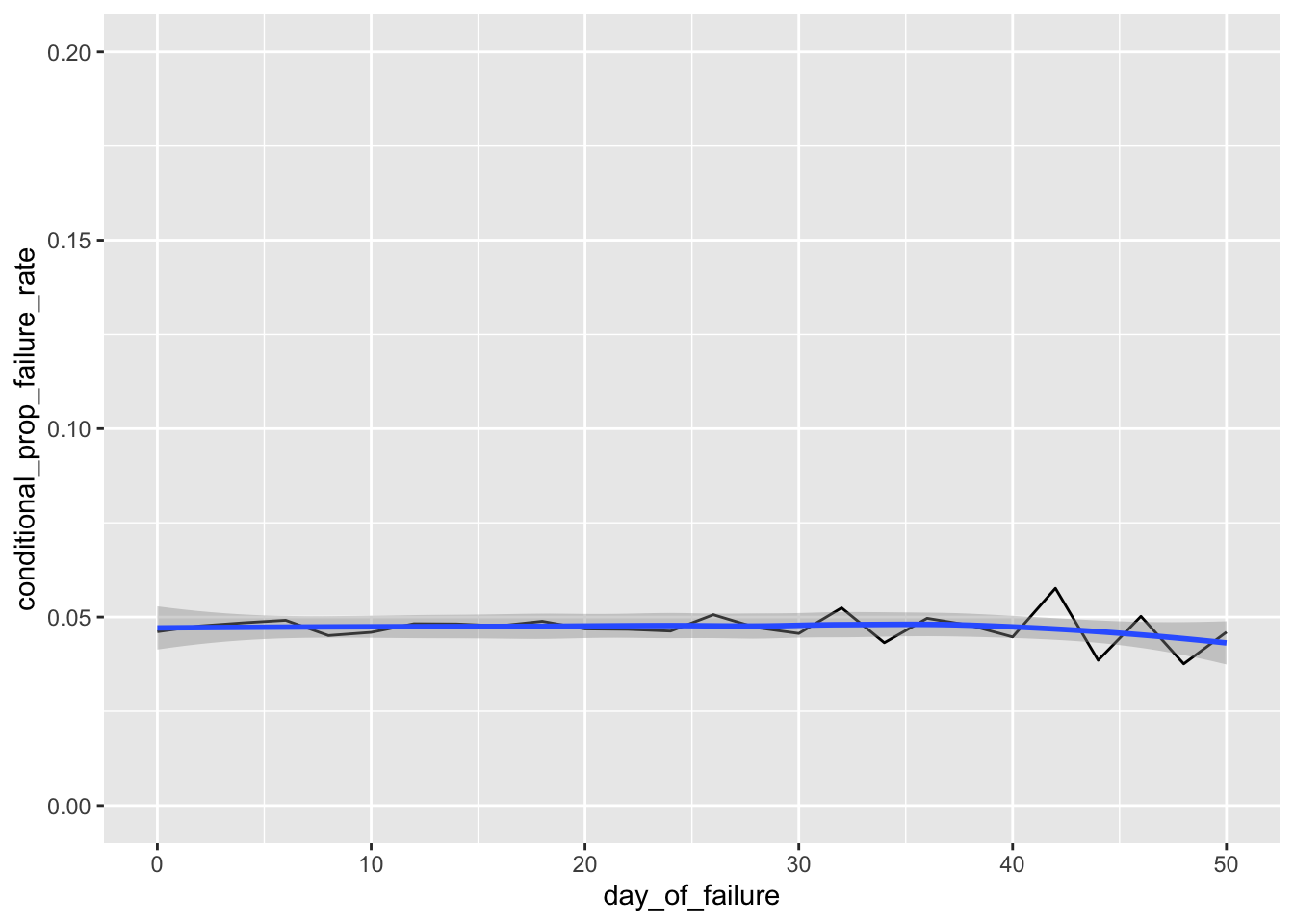

Of course, slicing by even days is arbitrary. Why don’t we do it by 1/10ths of a day instead to get a more detailed look at how the failures occur over time. Again, we will divide by the width of the interval to get the failure rate per day. Notice that we can compare these two rates because they have both been normalized to proportion of failures per day. Of course, we expect them to be the same.

\[ \frac{P(20 \leq T \lt 20.1 | T \geq 20)}{20.1 - 20} \]

# Calculate the counts of survivals and failures.
h_tenths <- data %>% group_by(time_of_failure=round(lifetime, 1)) %>%
  summarize(n_failed=n()) %>%
  mutate(n_survived = nrow(data) - cumsum(n_failed),
         n_started=lag(n_survived,1, default=nrow(data))) %>%
  select(time_of_failure, n_started, n_failed, n_survived)
# Change them into proportions - notice how we divide the conditional proportion  by the width of the interval to make it comparable with our previous plot
h_tenths <- h_tenths %>% mutate(prop_survived=n_survived / first(n_started), conditional_prop_failed=n_failed / (n_started ) / (1/10))

head(h_tenths)

## # A tibble: 6 x 6
##   time_of_failure n_started n_failed n_survived prop_survived conditional_prop_…
##             <dbl>     <int>    <int>      <int>         <dbl>              <dbl>
## 1             0       10000       20       9980         0.998             0.02  
## 2             0.1      9980       60       9920         0.992             0.0601
## 3             0.2      9920       39       9881         0.988             0.0393
## 4             0.3      9881       50       9831         0.983             0.0506
## 5             0.4      9831       52       9779         0.978             0.0529
## 6             0.5      9779       37       9742         0.974             0.0378

ggplot(h_tenths, aes(time_of_failure, prop_survived)) + geom_line() + ggtitle("Survivor Function")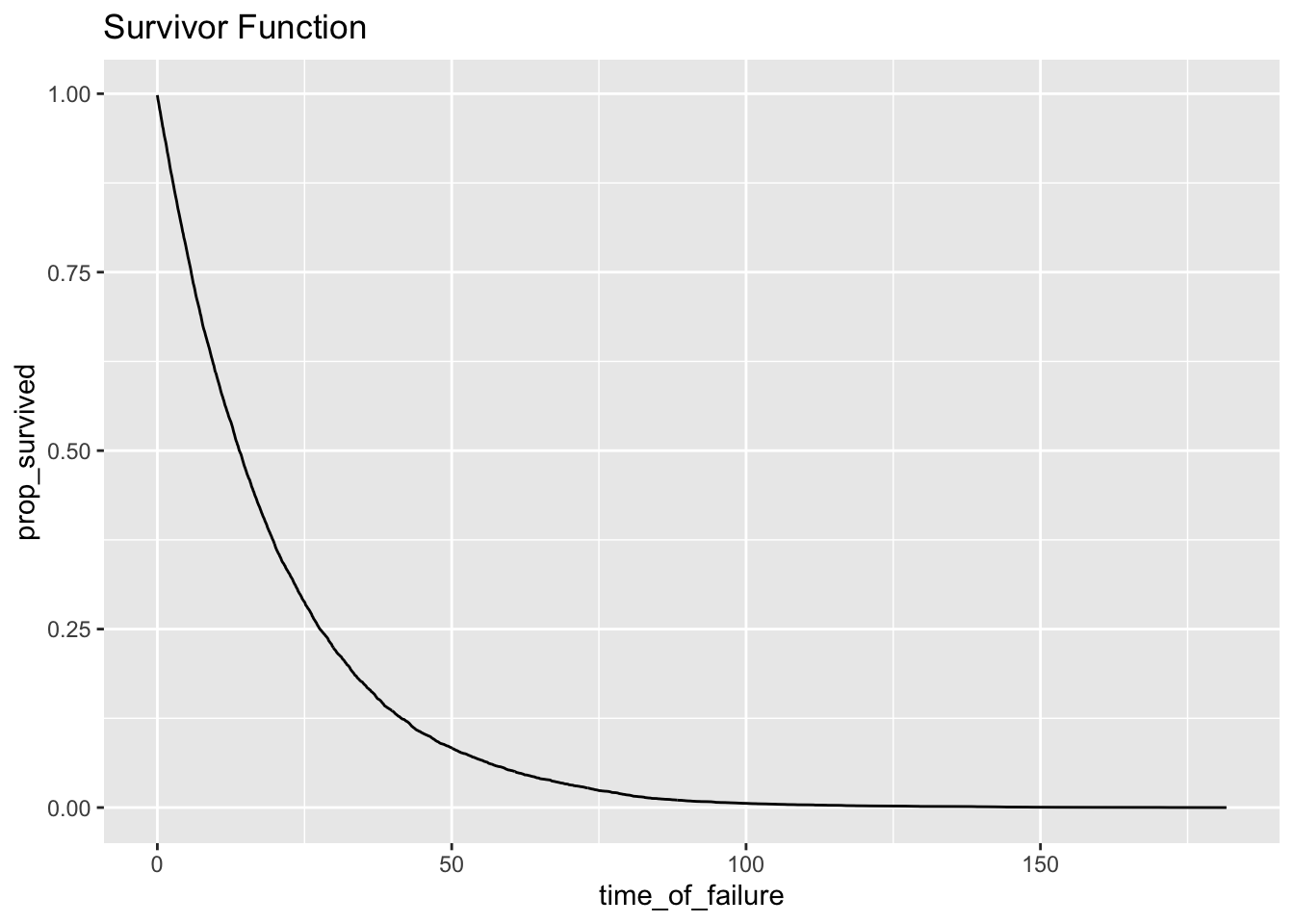

# Hazard Function
ggplot(h_tenths, aes(time_of_failure, conditional_prop_failed)) + geom_line() +
  xlim(0, 50) + ylim(0, .2) + geom_smooth(method='loess')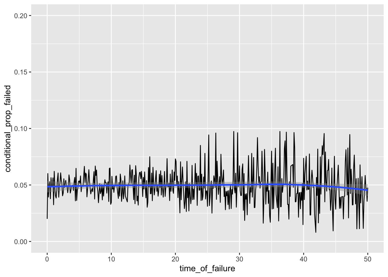

Now that we understand the process, there is no point in stopping at 1/10th of a day. We can keep slicing to finer time slices until they are infinitesimally small. This is what we will use as the hazard rate function.

\[ h(t) := \lim_{\delta \to 0}\frac{P(t \leq T \lt t + \delta | t \leq T )}{\delta} \] We can think of the hazard function as describing the risk accumulated for passing through each time point. As a chip goes through time, it picks up risk in proportion to the hazard function. At a certain point, enough risk accumulates and the component fails.

Relationship of hazard to other functions

In the previous section, we defined four functions to describe survival times: density, distribution, survivor and hazard. We will now look at how these four functions are intimately related. In fact, knowing one of the functions allows us to get at any of the other three.

Using some elementary definitions from probability, we will see that the hazard rate is just the density divided by the survivor: \[ h(t) = \frac{f(t)}{S(t)} \] Here is the derivation.

\[ \begin{align} h(t) & = \lim_{\delta \to 0}\frac{P(t \leq T \lt t + \delta | t \leq T )}{\delta} \\ & = \lim_{\delta \to 0}\frac{P(t \leq T \lt t + \delta)}{\delta P(t \leq T )} \tag{1} \\ & = \lim_{\delta \to 0}\frac{P(t \leq T \lt t + \delta)}{\delta S(t)} \\ & = \lim_{\delta \to 0}\frac{P(t \leq T \lt t + \delta)}{\delta } \frac{1}{S(t)} \\ & = \lim_{\delta \to 0} \frac{F(t+\delta) - F(t)}{\delta}\frac{1}{S(t)} \\ & = \frac{F'(t)}{S(t)} = \frac{f(t)}{S(t)} \tag{2} \end{align} \] (1) is from the definition of conditional probability. (2) is from the definition of a derivative, and the fact that the density function is the derivative of the distribution function.

Observations not starting at time 0

In real world data sets, we very seldomly observe subjects from the onset of risk at time 0. Instead, there is some starting time \(t_0 > 0\). In these cases, we can work with the conditional variants of our functions.

\[ h(t \mid T > t_0) = h(t) \\ H(t \mid T > t_0) = H(t) - H(t_0) \\ F(t \mid T > t_0) = \frac{F(t) - F(t_0)}{S(t_0)} \\ S(t \mid T > t_0) = \frac{S(t)}{S(t_0)} \]

Simulating failure times with quantile functions

A less common, but very useful, way to describe the data is the quantile function. These functions allow us to generate artificial datasets. Often denoted Q(u), a quantile function is defined as the inverse of the cumulative distribution function.

\[ Q(u) = F^{-1}(u) \]

Intuitively, given a proportion of failures, Q returns the time it takes to reach that proportion of failures.

We can use the [Probability Integral Transform], to simulate failure times given a hazard function. The transform tells us that passing draws of a random variable through its’ own distribution function results in a uniform random variable. We can also run this process in reverse and pass a uniform through the quantile (inverse cumulative) function.

For example, let’s take a look at failure times for a Weibull with p=3. Here is the cumulative distribution function, and its’ inverse:

\[ F(t) = 1 - exp(-t^3) \\ F^{-1}(u) = [-ln(1 - u)]^{1/3} \]

u = runif(n=5)
F_inv <- function(x) { (-log(1 - x))^(1/3)  }
t = F_inv(u)
t

## [1] 1.480 0.687 1.066 1.472 1.069

We can also describe the conditional distribution of failure times for when we start observing at some time t_0 that is not 0.

Using our definitions of conditional distributions above, we can derive the conditional quantile function for the Weibull.

\[ S(t \mid T > t_0) = \frac{S(t)}{S(t_0)} \\ F(t \mid T > t_0) = 1 - S(t \mid T > t_0) \\ = 1 - \frac{S(t)}{S(t_0)} \\ = 1 - \frac{exp(-t^p)}{exp(-t_0^p)} \]

Letting u be the quantile, let’s solve for t to get us the conditional quantile function \[ u = 1 - \frac{exp(-t^p)}{exp(-t_0^p)} \\ 1 - u = \frac{exp(-t^p)}{exp(-t_0^p)} \\ exp(-t_0^p)(1 - u) = exp(-t^p) \\ -t_0^p + ln(1 - u) = -t^p \\ t = (t_0^p - ln(1 - u))^\frac{1}{p} = Q(u) \]

Using our Q(u), we can simulate from the conditional distribution with t_0 = 2, and p=3

u = runif(n=5)
F_inv <- function(u) {(2^3 - log(1 - u))^(1/3)}
F_inv(u)

## [1] 2.13 2.05 2.04 2.01 2.03

We can use this conditional quantile function to generate repeated failures by conditioning on the previous failure time. That is, if a unit could fail repeatedly, then we would run a unit to failure and then restart the process so that each failure time is larger than the previous.

P <- 3
F_inv <- function(u, t0, p) {(t0^p - log(1 - u))^(1/p)}

u <- rep(NA, 5)
u[1] = F_inv(runif(1), 0, P)
for(i in 2:length(u)){
  u[i] <- F_inv(runif(1), u[i-1], P)
}

u

## [1] 0.82 1.06 1.28 1.31 1.63

Interpreting Cumulative Hazard

The cumulative hazard is much easier to interpret than the hazard. We can think of the cumulative hazard as the total amount of risk a component has picked up as it travels through time. As an analogy, imagine that you are walking along a path, and at each step you have to pick up a rock. These rocks start getting heavy as you go, until at some point you collapse of exhaustion. This is similar to how risk builds. Recall that \[ S(t) = exp(-H(t)) \] . So a cumulative hazard of 2 at some time point t means that the probability of making it past t is just 13.5%:

exp(-2)

## [1] 0.135

Another way to think about cumulative hazard is how many times we expect a single component to fail if it could fail multiple times. In this case, with H(t) = 2, we expect the same component to have failed twice. This is called the count data interpretation.

Going back to our example of the Weibull with p=3, we have the cumulative hazard function \(t^3\). That means the cumulative hazard at t=4 is 64, and so we expect a component that can fail repeatedly to do so 64 times.

Let’s carry out a simulation with our Weibull distribution.

P <- 3
F_inv <- function(u, t0, p) {(t0^p - log(1 - u))^(1/p)}

# Simulate a component that can fail multiple times. We go up to the nth failure. 
simulate <- function(n) {
  u <- rep(NA, n)
  u[1] = F_inv(runif(1), 0, P)
  for(i in 2:length(u)){
    u[i] <- F_inv(runif(1), u[i-1], P)
  }
u
}

set.seed(123)
data <- data.frame()
for(i in 1:1000){
  # We simulate up to 200 failures for each component to make sure we observe each component well past time 4.
  u <- simulate(n=200)
  # Count up the number of failures before t=4 for each simulation.
  count <- sum(u <= 4)
  data <- rbind(data, data.frame(sim=i, failures=count))
}
head(data)

##   sim failures
## 1   1       63
## 2   2       63
## 3   3       67
## 4   4       56
## 5   5       68
## 6   6       72

mean(data$failures)

## [1] 63.9

According to our count data interpretation, we expect the number of failures before t=4 to be t^3 = 64. Our simulation shows the mean number of failures to be 63.9, pretty darn close to our theoretical one.

That’s it! To recap, we have learned how we can use the density, distribution, survivor and hazard functions to describe failure times. From these four functions, we can derive the quantile function to simulate failures and cumulative hazard to interpret the average number of failures when repeated failures is allowed. Next time we will discuss how to estimate these functions in the presence of censored data.

For more, see Part 2 - KM Estimation.

Probability Integral Transformation

If a RV X is distributed according to some CDF, F. Then F(X) is the uniform.

For example, let X represent scores on a test. Plugging X into F will give back the percentile, that is the number of scores that were lower than X. Percentiles are uniformly distributed, that is there are as many people between the 1st and 2nd percentile as there are between the 49th and 50th. The CDF’s job is to exactly redistribute the test scores such that it is uniform over [0,1].

Proof: Let X by a continuous RV with CDF F_X, and let Y be a RV that comes from applying the CDF of a RV to itself. Then Y is a uniform over [0,1]. \[ F_Y(y) = P(Y \leq y) \\ = P(F_X(X) \leq y) \\ = P(X \leq F_X^{-1}(y)) \\ = F_X(F^{-1}_X(y)) \\ = y \] We recognize this as the CDF of Uniform(0,1)

We can use this fact in reverse. Given a uniform variable and a CDF, we can apply the inverse to get back the RV distributed according to that CDF.

If U is a uniformly distributed RV on [0,1], then Q(U) is a RV with cumulative distribution F.