In the previous section we discussed four functions used to describe failure times: density, distribution, survivor and hazard. In this section we will talk about how to estimate the survivor function, S(t), with the Kaplan-Meier method. After we obtain S(t), we will see how the log-rank test, a variant of the chi-square test, can be used to compare two different survivor functions.
Estimating the survivor function
Continuing with our example from last time, let’s revisit the failure times of our box of microchips.
set.seed(123)
# Let's say the mean lifetime of a component is 20 hours.
N = 100
mean_lifetime = 20
# Generate 100 component failures randomly
lifetimes <- rexp(n=N, rate=1/mean_lifetime)
data <- data.frame(lifetime = lifetimes)
# Let's take a look at the data.
head(data)
## lifetime
## 1 16.869
## 2 11.532
## 3 26.581
## 4 0.632
## 5 1.124
## 6 6.330data %>% summarize(mean_lifetime=mean(lifetime))## mean_lifetime
## 1 20.9# We won't have arbitrary precision in the real world, so let's bucket the data to day and truncate decimals.
data %>% group_by(coarse_lifetime=floor(lifetime)) %>%
summarize(n=n(), values=paste(round(lifetime, 2), collapse=",")) %>%
head(n=5)## # A tibble: 5 x 3
## coarse_lifetime n values
## <dbl> <int> <chr>
## 1 0 6 0.63,0.58,0.64,0.84,0.85,0.09
## 2 1 5 1.12,1.81,1.97,1.97,1.35
## 3 2 1 2.91
## 4 3 1 3.77
## 5 4 3 4.51,4.77,4.32Counting method
In order to estimate S(t), we will first organize the data into a particular table format. The observed failure times failure times are ordered from smallest to largest to create “bins”. Then each row represents one bin with the at-risk count being the number of units that made it to the start of the bin, and failed + censored being the number removed. S(t) is the proportion of units that make it to the start of the next time period as a fraction of the total.
Here is the table for the first few rows:
| time | at-risk | failed | censored | S(t) |
|---|---|---|---|---|
| - | 100 | 0 | 0 | 1 |
| 0 | 100 | 6 | 0 | .94 |
| 1 | 94 | 5 | 0 | .89 |
| 2 | 89 | 1 | 0 | .88 |
| 3 | 88 | 1 | 0 | .87 |
Let’s do this programmatically for all the entire dataset.
km_table <- data %>% group_by(coarse_lifetime=floor(lifetime)) %>%
  summarize(n=n(), values=paste(round(lifetime, 2), collapse=",")) %>%
  mutate(tot_failed = cumsum(n), S=(N-tot_failed) / N) %>%
  mutate(at_risk=N-lag(tot_failed, n=1, default=0))  %>%
  select(t=coarse_lifetime, at_risk, failed=n, tot_failed, S)
## `summarise()` ungrouping output (override with `.groups` argument)km_table## # A tibble: 41 x 5
## t at_risk failed tot_failed S
## <dbl> <dbl> <int> <int> <dbl>
## 1 0 100 6 6 0.94
## 2 1 94 5 11 0.89
## 3 2 89 1 12 0.88
## 4 3 88 1 13 0.87
## 5 4 87 3 16 0.84
## 6 5 84 7 23 0.77
## 7 6 77 5 28 0.72
## 8 7 72 2 30 0.7
## 9 8 70 1 31 0.69
## 10 9 69 4 35 0.65
## # … with 31 more rowsKaplan-Meier method
An alternative way to estimate S is to multiply a series of conditional probabilities. Intuitively, for a component to have a failure time greater than two it must survive three rounds of culling (t=0, t=1, and t=2).
\[ \begin{align} S(2) & = P(T > 2) \\ & = P(T \geq 0) * P(T > 0 | T \geq 0) * P(T > 1 | T \geq 1) * P(T > 2 | T \geq 2) \\ & = 1 * \frac{100-6}{100} * \frac{94-5}{94} * \frac{89 - 1}{89} \\ & = .94 * .947 * .989 = .88 \end{align} \] The conditional probabilities here look slightly unusual here. Intuitively, for each bucket we want to count the number of units that failed within a time bucket as a proportion of units that made it to the start of the bucket. For an elementary proof of this result, see Appendix.
Notice that this aligns exactly with our previous counting solution.
Dealing with censoring
Next, we add censoring back into the mix starting with the same simulated dataset as before.
set.seed(123)
# Let's say the mean lifetime of a component is 20 hours.
N = 100
mean_lifetime = 20
# Generate 100 component failures randomly
lifetimes <- rexp(n=N, rate=1/mean_lifetime)
# Draw 100 bernoulli variables deciding which observations will get censored.
censored <- rbernoulli(n=N, p=.2)
# Draw 100 censoring times from 0 up to the lifetime of the component.
censored_time <- map_dbl(lifetimes, ~ runif(n=1, min=0, max=.))
data_censored <- data.frame(lifetime=lifetimes, censored, censored_time, lifetime_censored = ifelse(censored, censored_time, lifetimes))

# Let's take a look at the data.
head(data_censored)
## lifetime censored censored_time lifetime_censored
## 1 16.869 TRUE 1.216 1.216
## 2 11.532 FALSE 1.894 11.532
## 3 26.581 FALSE 20.476 26.581
## 4 0.632 FALSE 0.464 0.632
## 5 1.124 FALSE 1.093 1.124
## 6 6.330 FALSE 2.953 6.330data_censored %>% summarize(mean_lifetime=mean(lifetime))## mean_lifetime
## 1 20.9# Drop the temporary columns used for censoring.
data_censored <- data_censored %>% select(lifetime=lifetime_censored, censored=censored)
# We won't have arbitrary precision in the real world, so let's bucket the data to the nearest hour.
data_censored %>% group_by(coarse_lifetime=floor(lifetime)) %>%
summarize(n=n(), values=paste(round(lifetime, 2), collapse=",")) %>%
head(n=5)## `summarise()` ungrouping output (override with `.groups` argument)## # A tibble: 5 x 3
## coarse_lifetime n values
## <dbl> <int> <chr>
## 1 0 8 0.63,0.47,0.58,0.64,0.11,0.84,0.85,0.09
## 2 1 9 1.22,1.12,1.71,1.21,1.81,1.97,1.26,1.85,1.35
## 3 2 3 2.91,2.14,2.19
## 4 3 1 3.77
## 5 4 3 4.51,4.32,4.21Again, we will construct our KM table, but this time taking censoring into account.
km_table_censored <- data_censored %>%
  group_by(coarse_lifetime=floor(lifetime)) %>%
  # Count the number of failures and censored separately.
  summarize(failures=sum(ifelse(!censored, 1, 0)), censored=sum(ifelse(censored, 1, 0))) %>%
  mutate(failed_or_censored = failures + censored,
         tot_removed=cumsum(failed_or_censored),
         at_risk=N-lag(tot_removed, 1, 0),
         survival_rate = 1 - (failures / at_risk),
         S=cumprod(survival_rate))
## `summarise()` ungrouping output (override with `.groups` argument)km_table_censored## # A tibble: 41 x 8
## coarse_lifetime failures censored failed_or_censo… tot_removed at_risk
## <dbl> <dbl> <dbl> <dbl> <dbl> <dbl>
## 1 0 6 2 8 8 100
## 2 1 4 5 9 17 92
## 3 2 1 2 3 20 83
## 4 3 1 0 1 21 80
## 5 4 2 1 3 24 79
## 6 5 5 2 7 31 76
## 7 6 4 2 6 37 69
## 8 7 2 1 3 40 63
## 9 8 1 0 1 41 60
## 10 9 2 2 4 45 59
## # … with 31 more rows, and 2 more variables: survival_rate <dbl>, S <dbl># Let's clean it up a bit
km_table_censored <- km_table_censored %>% select(t=coarse_lifetime, at_risk, failures, censored, S)
km_table_censored## # A tibble: 41 x 5
## t at_risk failures censored S
## <dbl> <dbl> <dbl> <dbl> <dbl>
## 1 0 100 6 2 0.94
## 2 1 92 4 5 0.899
## 3 2 83 1 2 0.888
## 4 3 80 1 0 0.877
## 5 4 79 2 1 0.855
## 6 5 76 5 2 0.799
## 7 6 69 4 2 0.752
## 8 7 63 2 1 0.729
## 9 8 60 1 0 0.716
## 10 9 59 2 2 0.692
## # … with 31 more rowsd1 <- km_table %>% mutate(method="count") %>% select(t, S, method)
d2 <- km_table_censored %>% mutate(method="product") %>% select(t, S, method)
d3 <- km_table_censored_is_failure %>% mutate(method="censor_is_failure") %>% select(t, S, method)
d4 <- km_table_censored_ignored %>% mutate(method="censor_ignored") %>% select(t, S, method)
d <- rbind(d1, d2, d3, d4)
ggplot(d, aes(t, S, colour=method)) + geom_line() + ggtitle("S(t) by various estimation methods")
We can immediately see that ignoring censored values lead to a very inaccurate survival curve. Surprisingly, treating censored time as failure time results in a pretty accurate survival curve. However, this will consistently underestimate the true curve and the problem only gets worse with more censoring. The KM method was developed to address these issues, and does a pretty good job of approximating the true survival curve here.
Log rank test for comparing survival functions
Now that we can estimate the survivor function, we’d like to ask whether two survival curves are equivalent. Since we are dealing with estimates of survivor functions, we ask this question with hypothesis testing.
Given two groups, we can compare their survival curves using the log rank test (Peto 1977). The log-rank test is a chi-square test that compares the observed failure counts to expected failure counts.
At some time t, the expected failures in a group is the total number of failures at t multiplied by the proportion at risk for that group.
Here is a dataset of lukemia patients which consideres relapse a failure:
tx <- data.frame(lifetime=c(6,6,6,7,10,13,16,22,23,6,9,10,11,17,19,20,25,32,32,34,35),
                 censored=c(rep(FALSE,9), rep(TRUE, 12)),
                 group="tx")
ctl <- data.frame(lifetime=c(1,1,2,2,3,4,4,5,5,8,8,8,8,11,11,12,12,15,17,22,23),
                  censored=c(rep(FALSE, 21)),
                  group="ctl")

# Pool the data, calculate at-risk / failures per time point in each group.
data <- rbind(tx, ctl)
data <- data %>% arrange(lifetime)
# Initialize the at-risk columns to the group sizes.
data$at_risk_ctl = NA;  data$at_risk_ctl[1] <- nrow(ctl)
data$at_risk_tx = NA; data$at_risk_tx[1] <- nrow(tx)
# Initialize the failed columns to 0
data$failed_ctl = 0; data[1,]$failed_ctl = ifelse(data[1,]$group == 'ctl' && !data[1,]$censored,1,0)
data$failed_tx = 0; data[1,]$failed_tx = ifelse(data[1,]$group == 'tx' && !data[1,]$censored,1,0)
for(i in 2:nrow(data)){
  # Always subtract from at_risk, whether censored or failed.
  data[i,]$at_risk_ctl = data[i-1,]$at_risk_ctl - ifelse(data[i-1,]$group == 'ctl',1,0)
  data[i,]$at_risk_tx = data[i-1,]$at_risk_tx - ifelse(data[i-1,]$group == 'tx',1,0)
  # Only add to failed if the data was not censored
  data[i,]$failed_ctl= ifelse(data[i,]$group == 'ctl' && !data[i,]$censored,1,0)
  data[i,]$failed_tx= ifelse(data[i,]$group == 'tx' && !data[i,]$censored,1,0)
}

# Group by lifetimes
data <- data %>% group_by(lifetime) %>%
  summarize(failed_ctl = sum(failed_ctl),
            failed_tx=sum(failed_tx),
            at_risk_ctl=max(at_risk_ctl),
            at_risk_tx=max(at_risk_tx))
## `summarise()` ungrouping output (override with `.groups` argument)# Calculate expected failures per row.
data$expected_failed_ctl <- data$at_risk_ctl / (data$at_risk_tx + data$at_risk_ctl) * (data$failed_ctl + data$failed_tx)
data$expected_failed_tx <- data$at_risk_tx / (data$at_risk_tx + data$at_risk_ctl) * (data$failed_ctl + data$failed_tx)
data$diff_ctl = data$failed_ctl - data$expected_failed_ctl
data$diff_tx = data$failed_tx - data$expected_failed_tx
head(data)## # A tibble: 6 x 9
## lifetime failed_ctl failed_tx at_risk_ctl at_risk_tx expected_failed…
## <dbl> <dbl> <dbl> <dbl> <dbl> <dbl>
## 1 1 2 0 21 21 1
## 2 2 2 0 19 21 0.95
## 3 3 1 0 17 21 0.447
## 4 4 2 0 16 21 0.865
## 5 5 2 0 14 21 0.8
## 6 6 0 3 12 21 1.09
## # … with 3 more variables: expected_failed_tx <dbl>, diff_ctl <dbl>,
## # diff_tx <dbl># Take the sum of a group, say ctl, as our statistic
total_diff <- sum(data$diff_ctl)
# Formula for variance of the expected difference - See Kleinbaum and Klein p70.
s = 0
# Skip the last row which causes division by 0.
for(i in 1:nrow(data[-1,])) {
at_risk_tx <- data[i,]$at_risk_tx
at_risk_ctl <- data[i,]$at_risk_ctl
failed_tx <- data[i,]$failed_tx
failed_ctl <- data[i,]$failed_ctl
s = s + (
((at_risk_ctl * at_risk_tx * (failed_ctl + failed_tx) * (at_risk_ctl + at_risk_tx - failed_ctl - failed_tx))) /
((at_risk_ctl + at_risk_tx)^2 * (at_risk_ctl + at_risk_tx - 1)))
}
diff_var <- s
log_rank_statistic <- total_diff^2 / diff_var
sprintf("Log rank statistic: %.1f", log_rank_statistic)## [1] "Log rank statistic: 16.8"# Look up our statistic. Shows that the p-value is pretty much 0.
pchisq(log_rank_statistic, df=1, lower.tail=F)## [1] 4.17e-05For each group, the method calculates at each event time the number of events one would expect since the previous event if there were no differences in the groups.
The R implementation is much simpler and yields the same results.
library(survival)## Warning: package 'survival' was built under R version 4.0.2tx <- data.frame(lifetime=c(6,6,6,7,10,13,16,22,23,6,9,10,11,17,19,20,25,32,32,34,35),
death=c(rep(TRUE,9), rep(FALSE, 12)),
group="tx")
ctl <- data.frame(lifetime=c(1,1,2,2,3,4,4,5,5,8,8,8,8,11,11,12,12,15,17,22,23),
death=c(rep(TRUE, 21)),
group="ctl")
lukemia <- rbind(tx, ctl)
# Fit survival curve
fit <- survfit(Surv(lifetime, death) ~ group, data=lukemia)
print(fit)## Call: survfit(formula = Surv(lifetime, death) ~ group, data = lukemia)
##
## n events median 0.95LCL 0.95UCL
## group=ctl 21 21 8 4 12
## group=tx 21 9 23 16 NAsummary(fit)## Call: survfit(formula = Surv(lifetime, death) ~ group, data = lukemia)
##
## group=ctl
## time n.risk n.event survival std.err lower 95% CI upper 95% CI
## 1 21 2 0.9048 0.0641 0.78754 1.000
## 2 19 2 0.8095 0.0857 0.65785 0.996
## 3 17 1 0.7619 0.0929 0.59988 0.968
## 4 16 2 0.6667 0.1029 0.49268 0.902
## 5 14 2 0.5714 0.1080 0.39455 0.828
## 8 12 4 0.3810 0.1060 0.22085 0.657
## 11 8 2 0.2857 0.0986 0.14529 0.562
## 12 6 2 0.1905 0.0857 0.07887 0.460
## 15 4 1 0.1429 0.0764 0.05011 0.407
## 17 3 1 0.0952 0.0641 0.02549 0.356
## 22 2 1 0.0476 0.0465 0.00703 0.322
## 23 1 1 0.0000 NaN NA NA
##
## group=tx
## time n.risk n.event survival std.err lower 95% CI upper 95% CI
## 6 21 3 0.857 0.0764 0.720 1.000
## 7 17 1 0.807 0.0869 0.653 0.996
## 10 15 1 0.753 0.0963 0.586 0.968
## 13 12 1 0.690 0.1068 0.510 0.935
## 16 11 1 0.627 0.1141 0.439 0.896
## 22 7 1 0.538 0.1282 0.337 0.858
## 23 6 1 0.448 0.1346 0.249 0.807plot(fit, col=1:2, xscale=7, lwd=2, mark.time=TRUE,
xlab="Weeks since study entry", ylab="Survival")
legend(21, .9, c("Control", "Treatment"), col=1:2, lwd=2, bty='n')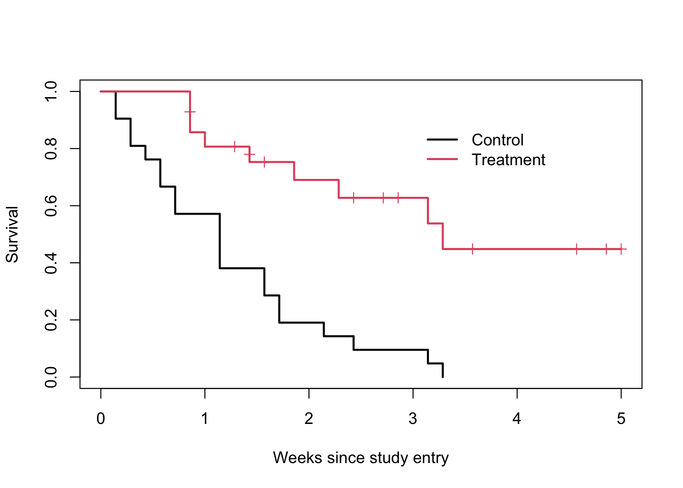
# Log rank test
survdiff(Surv(lifetime, death) ~ group, data=lukemia)
## Call:
## survdiff(formula = Surv(lifetime, death) ~ group, data = lukemia)
##
## N Observed Expected (O-E)^2/E (O-E)^2/V
## group=ctl 21 21 10.7 9.77 16.8
## group=tx 21 9 19.3 5.46 16.8
##
## Chisq= 16.8 on 1 degrees of freedom, p= 4e-05Next time
In this post, we discussed KM survival curves and the logrank test. Both are useful for investigating how a single factor affects survival. While useful in experimental studies, we will see many situations where several factors may affect the outcome. For example, the two groups under study might have a large difference in age. To analyze these situations, we must reach for more sophisticated methods.
In the next part, we will discuss the Cox proportional hazards model which accounts for covariates at the time of study entry. The Cox PH model uses a regression framework to estimate the hazard function based on entry covariates.
Appendix
Proof of KM estimator
Let S(t) be the survivor function, and \(t_{(f)}\) be the ordered failure times. For example, \(t_{(1)}\) is the first failure and $t_{(N)} is the last failure time.
Recall that \[ S(t) = Pr(T > t_{(f)}) \]
Let’s expand the right hand side to include an extra condition that doesn’t change the probability: \[ S(t) = Pr(T \geq t_{(f)}, T > t_{(f)}) \] We can do this because the first event contains the second one. Intuitively, think about rolling a die and asking for the probability it comes up six. This is the same probability as the die coming up six and even.
Using the definition of a joint probability, we have: \[ \begin{align} S(t) & = Pr(T \geq t_{(f)}, T > t_{(f)}) \\ & = Pr(T \geq t_{(f)}) * Pr(T > t_{(f)} \mid T \geq t_{(f)}) \end{align} \] Since we ordered failure times, there are no failures between \(t_{(f-1)}\) and \(t_{(f)}\) so \[ Pr(T > t_{(f-1)}) = Pr(T \geq t_{(f)}) \]
Therefore \[ \begin{align} &Pr(T \geq t_{(f)}) * Pr(T > t_{(f)} \mid T \geq t_{(f)}) \\ & = Pr(T > t_{(f-1)}) * Pr(T > t_{(f)} \mid T \geq t_{(f)}) \\ & = S(t_{(f-1)}) * Pr(T > t_{(f)} \mid T \geq t_{(f)}) \end{align} \]