There are three statistical objectives for a survival model:
- Test for significance of the treatment variable.
- Obtain a point estimate of the effect.
- Obtain a confidence interval for the effect.
The Cox proportional hazard (PH) model captures how the hazard function is modified by covariates.
\[ h(t, X) = h_0(t) e^{\sum_i^p \beta_i X_i} \]
We exponentiate a linear function of X to ensure that the entire hazard function stays non-negative.
Notice that the baseline hazard, \(h_0\), is a function of t only, and the multiplier \(exp(\sum \beta_i X_i)\) is a function of X only. This implies that the covariates are time-independent. Time independent variables are variables whose value for a given individual does not change over time. Examples are sex, and smoking status. It is possible to model time-dependent covariates, but those models are called extended Cox models.
When all the covariates are 0, the Cox formula collapses into just the baseline hazard. Thus, \(h_0(t)\) can be interpreted as the starting point before taking any covariates into account.
Note that \(h_0(t)\) is unspecified, making this a semi-parametric model. Fortunately, can still estimate the covariate \(\beta\)’s, the quantities of interest, without specifying a baseline hazard model.
Here is an example fit of a Cox PH model.
tx <- data.frame(lifetime=c(6,6,6,7,10,13,16,22,23,6,9,10,11,17,19,20,25,32,32,34,35),
                 log_wbc=c(2.31, 4.06, 3.28, 4.43, 2.96, 2.88, 3.60, 2.32, 2.57, 3.20, 2.80, 2.70, 2.60, 2.16, 2.05, 2.01, 1.78, 2.20, 2.53, 1.47, 1.45),
                 death=c(rep(TRUE,9), rep(FALSE, 12)),
                 group="tx",
                 ctl=0)
ctl <- data.frame(lifetime=c(1,1,2,2,3,4,4,5,5,8,8,8,8,11,11,12,12,15,17,22,23),
                  log_wbc=c(2.80, 5.00, 4.91, 4.48, 4.01, 4.36, 2.42, 3.49, 3.97, 3.52, 3.05, 2.32, 3.26, 3.49, 2.12, 1.50, 3.06, 2.30, 2.95, 2.73, 1.97),
                  death=c(rep(TRUE, 21)),
                  group="ctl",
                  ctl=1)
lukemia <- rbind(tx, ctl)
head(lukemia)
## lifetime log_wbc death group ctl
## 1 6 2.31 TRUE tx 0
## 2 6 4.06 TRUE tx 0
## 3 6 3.28 TRUE tx 0
## 4 7 4.43 TRUE tx 0
## 5 10 2.96 TRUE tx 0
## 6 13 2.88 TRUE tx 0lukemia_fit <- coxph(Surv(lifetime, death) ~ ctl + log_wbc, data=lukemia)
summary(lukemia_fit)## Call:
## coxph(formula = Surv(lifetime, death) ~ ctl + log_wbc, data = lukemia)
##
## n= 42, number of events= 30
##
## coef exp(coef) se(coef) z Pr(>|z|)
## ctl 1.386 3.999 0.425 3.26 0.0011 **
## log_wbc 1.691 5.424 0.336 5.03 4.8e-07 ***
## ---
## Signif. codes: 0 '***' 0.001 '**' 0.01 '*' 0.05 '.' 0.1 ' ' 1
##
## exp(coef) exp(-coef) lower .95 upper .95
## ctl 4.00 0.250 1.74 9.2
## log_wbc 5.42 0.184 2.81 10.5
##
## Concordance= 0.852 (se = 0.04 )
## Likelihood ratio test= 46.7 on 2 df, p=7e-11
## Wald test = 33.6 on 2 df, p=5e-08
## Score (logrank) test = 46.1 on 2 df, p=1e-10Hazard Ratio
Results from a Cox PH regression are often reported as a hazard ratio (HR). Intuitively, hazard ratios are scaling factor between two risk profiles based on various measured factors.
The HR between some individual whose covariates are denoted X and some other individual, X*, is:
\[ \frac{h(t, X*)}{h(t, X)} \] It is easier to interpret HRs greater than 1, so covariates are often coded as 1 for the higher risk groups by convention.
\[ \begin{align} HR & = \frac{h(t, X*)}{h(t, X)} \\ & = \frac{h_0(t) e^{\sum_i^p \beta_i X^*_i}}{h_0(t) e^{\sum_i^p \beta_i X_i}} \\ & = \frac{e^{\sum_i^p \beta_i X^*_i}}{e^{\sum_i^p \beta_i X_i}} \\ & = e^{\sum_i^p \beta_i (X^*_i - X_i)} \\ & = exp\left(\sum_i^p \beta_i (X^*_i - X_i)\right) \\ \end{align} \] Notice how the \(h_0\) cancels out. If two individuals have the same covariates, then their HR is 1 and both are subject to an equal risk of failure.
Going back to our lukemia fit example, let’s calculate the HRs.
lukemia_fit <- coxph(Surv(lifetime, death) ~  ctl + log_wbc, data=lukemia)

# HR for two individuals that only differ by treatment, but have the same log WBC
tx_beta <- lukemia_fit$coefficients["ctl"]
exp(tx_beta)
## ctl
## 4This hazard ratio of 4 between individuals who are in the treatment group versus placebo. Notice that we did not use the coefficient for log WBC in this computation because it canceled out. Implicitly, we are comparing the survival of an individual if she had been assigned to treatment versus placebo. Since our hypothetical person would have the same log WBC count in either scenario, the terms cancel and we can safely drop it out of the computation.
To get the confidence interval for a HR, we simply take the standard 95% CI for regression coefficients and exponentiate it:
\[ exp\left[ \beta_1 \pm 1.96 \sqrt{Var(\beta_1)} \right] \]
s <- summary(lukemia_fit)

ctl_coef <- s$coefficients["ctl", "coef"]
ctl_se <- s$coefficients["ctl", "se(coef)"]
exp(c(ctl_coef + qnorm(.025) * ctl_se, ctl_coef + qnorm(.975)*ctl_se))
## [1] 1.74 9.20# CHECK: We can also just extract it directly from the fit object
s$conf.int## exp(coef) exp(-coef) lower .95 upper .95
## ctl 4.00 0.250 1.74 9.2
## log_wbc 5.42 0.184 2.81 10.5Interaction Effects
When there are interaction effects, our calculation becomes a bit more complicated. Let’s say we have reason to suspect that the treatment’s efficacy is modulated by white blood cell count. We can capture this hypothesis by including it as an interaction effect in our model.
lukemia_fit_interaction <- coxph(Surv(lifetime, death) ~  ctl + log_wbc + ctl:log_wbc, data=lukemia)
summary(lukemia_fit_interaction)
## Call:
## coxph(formula = Surv(lifetime, death) ~ ctl + log_wbc + ctl:log_wbc,
## data = lukemia)
##
## n= 42, number of events= 30
##
## coef exp(coef) se(coef) z Pr(>|z|)
## ctl 2.375 10.750 1.705 1.39 0.16
## log_wbc 1.872 6.504 0.451 4.15 3.4e-05 ***
## ctl:log_wbc -0.318 0.728 0.526 -0.60 0.55
## ---
## Signif. codes: 0 '***' 0.001 '**' 0.01 '*' 0.05 '.' 0.1 ' ' 1
##
## exp(coef) exp(-coef) lower .95 upper .95
## ctl 10.750 0.093 0.38 304.16
## log_wbc 6.504 0.154 2.69 15.75
## ctl:log_wbc 0.728 1.374 0.26 2.04
##
## Concordance= 0.851 (se = 0.041 )
## Likelihood ratio test= 47.1 on 3 df, p=3e-10
## Wald test = 32.4 on 3 df, p=4e-07
## Score (logrank) test = 49.9 on 3 df, p=9e-11Looking at the p-value, it looks like we do not have a good evidence for the interaction. But for illustrative purposes let’s keep going.
If we expand our definition of HR for our lukemia example, we would have: \[ \begin{align} HR(WBC) & = exp\left(\sum_i^p \beta_i (X^*_i - X_i)\right) \\ & = exp\left(\beta_{treatment} (1 - 0) + \beta_{logWBC}(log WBC - log WBC) + \beta_{interaction}(1*logWBC - 0 * logWBC)\right) \\ & = exp\left(\beta_{treatment} + \beta_{interaction}(logWBC)\right) \\ \end{align} \]
If interaction terms are present, the hazard ratio computation includes the treatment coefficient and interaction coefficients that contain the treatment.
Note that our HR is no longer the same for all individuals, and instead depends on the individual’s WBC measurement.
Interaction effects complicate the procedure for obtaining a confidence interval. Due to how the terms appear, the general formula for CIs require a coefficient variance-covariance matrix. The exact formula is beyond the scope of this presentation, but see Kleinbaum and Klein (p119) for more details.
summary(lukemia_fit_interaction)## Call:
## coxph(formula = Surv(lifetime, death) ~ ctl + log_wbc + ctl:log_wbc,
## data = lukemia)
##
## n= 42, number of events= 30
##
## coef exp(coef) se(coef) z Pr(>|z|)
## ctl 2.375 10.750 1.705 1.39 0.16
## log_wbc 1.872 6.504 0.451 4.15 3.4e-05 ***
## ctl:log_wbc -0.318 0.728 0.526 -0.60 0.55
## ---
## Signif. codes: 0 '***' 0.001 '**' 0.01 '*' 0.05 '.' 0.1 ' ' 1
##
## exp(coef) exp(-coef) lower .95 upper .95
## ctl 10.750 0.093 0.38 304.16
## log_wbc 6.504 0.154 2.69 15.75
## ctl:log_wbc 0.728 1.374 0.26 2.04
##
## Concordance= 0.851 (se = 0.041 )
## Likelihood ratio test= 47.1 on 3 df, p=3e-10
## Wald test = 32.4 on 3 df, p=4e-07
## Score (logrank) test = 49.9 on 3 df, p=9e-11cov_matrix <- vcov(lukemia_fit_interaction)
ctl_coef <- coef(lukemia_fit_interaction)["ctl"]
interaction_coef <- coef(lukemia_fit_interaction)["ctl:log_wbc"]
var_ctl <- cov_matrix["ctl", "ctl"]
var_interaction <- cov_matrix["ctl:log_wbc", "ctl:log_wbc"]
cov_ctl_wbc <- cov_matrix["ctl", "ctl:log_wbc"]
# HR is now a function of log_wbc, so let's say it's 2
log_wbc <- 2
l <- ctl_coef + log_wbc * interaction_coef
hr <- exp(ctl_coef + log_wbc * interaction_coef)
var_hr <- var_ctl + log_wbc^2 * var_interaction + 2 * log_wbc * cov_ctl_wbc
print("Interaction HR and CI for Log WBC=2")## [1] "Interaction HR and CI for Log WBC=2"c(hr, exp(l + c(-1, 1) * qnorm(.975) * sqrt(var_hr)))## ctl
## 5.70 1.35 24.04log_wbc <- 4
l <- ctl_coef + log_wbc * interaction_coef
hr <- exp(ctl_coef + log_wbc * interaction_coef)
var_hr <- var_ctl + log_wbc^2 * var_interaction + 2 * log_wbc * cov_ctl_wbc
print("Interaction CI for Log WBC=4")## [1] "Interaction CI for Log WBC=4"c(hr, exp(l + c(-1, 1) * qnorm(.975) * sqrt(var_hr)))## ctl
## 3.019 0.899 10.141Adjusted Survival Curves with the Cox Model
The two primary artifacts of survival analysis are hazard ratios and survival curves. When we don’t have additional covariates, we use the KM method to estimate a survival curve for each group. With covariates, we can use the Cox PH model, to adjust survival curves for various predictors.
Let \[ h(t, X) = h_0(t) exp(\sum_i^p \beta_i X_i) \] using the relationships between the various descriptors of survival time, we obtain \[ S(t, X) = S_0(t)^{exp(\sum_i^p \beta_i X_i)} \] Going back to our example without interaction effects, we will fit and plot each treatment group’s survival curve adjusted for log WBC. R will automatically use the mean of the exposure (e.g log_WBC), for both groups.
lukemia_fit <- coxph(Surv(lifetime, death) ~  ctl + log_wbc, data=lukemia)
dummy <- expand.grid(ctl=c(1, 0), log_wbc=mean(lukemia$log_wbc))
surv <- survfit(lukemia_fit, newdata=dummy)
plot(surv, col=1:2)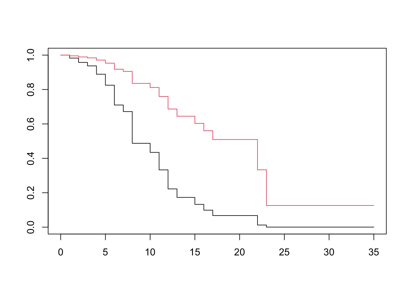
Appendix
Cox PH Likelihood
The standard formulation of the likelihood relies upon the joint probability distribution of all observations. We cannot do this with the Cox PH model because the base hazard function is left unspecified. Instead, the Cox likelihood is based on the order of observed events.
Imagine that three co-workers, Gary, Barry and Larry, enter a company lottery. Tickets are given out based on hours worked, so Barry receives 4 tickets, Gary receives 2 and Larry receives 1. Each employee can only win once, and the lottery is drawn once a week until everyone has won something.
Say that we observe the following oder of winners: Barry, Gary, then Larry. What is the probablity of this ordering?
Since the chances of winning are proportional to the tickets, we compute it as follows: \[ \frac{4}{7} \times \frac{2}{3} \times \frac{1}{1} = \frac {8}{21} \] Similarly, we can use the hazard function for various individuals to compute the likelihood of an ordering of failures. Imagine that instead of lottery tickets, we had failure times and smoker status.
| Patient | Failure Time | Status | Smoker |
|---|---|---|---|
| Barry | 2 | 1 | 1 |
| Gary | 3 | 1 | 1 |
| Harry | 5 | 0 | 0 |
| Larry | 8 | 1 | 0 |
If our model only had smoker as a covariate, the hazard function for a smoker would be \[ h_0(t)e^\beta \]
where \(h_0(t) e^0 = h_0(t)\) is the hazard for a non-smoker.
Plugging this into our likelihood, we would get \[ \begin{align} L &= \frac{h_0(t)e^\beta}{h_0(t)e^\beta + h_0(t)e^\beta + h_0(t) + h_0(t)} \\ & \times \frac{h_0(t)e^\beta}{h_0(t)e^\beta + h_0(t) + h_0(t)} \\ & \times \frac{h_0(t)}{h_0(t)} \end{align} \]
Factoring out the \(h_0(t)\), we get the likelihood’s reduced form. \[ L = \frac{e^\beta}{e^\beta + e^\beta + 1 + 1} \times \frac{e^\beta}{e^\beta + 1 + 1} \times \frac{1}{1} \]
With the likelihood in hand, we obtain the coefficients by maximization. This is done by taking the partial derivatives, setting them to 0 and solving the resulting system of equations.
Using Age as the Time Scale
Left Truncation and Left Censoring
Censoring occurs when we have unknown values because they occur outside the boundaries of our instruments. This can be due to either the instrument, e.g our water sensor cannot measure anything below 5 parts-per-million, or the design of the experiment itself (e.g a student cannot score higher than 100%, so their abilities are unbounded to the high side).
Truncation occurs when values outside our boundaries are excluded when gathered, or excluded when analyzed. For example, if a person conducting a survey asks for your income, and if you say anything higher than 100,000 they hang up, then you have been truncated. Truncation is an exclusion criteria.
Simply put, censored individuals show up in our dataset but we are unsure as to their exact value. Truncated individuals do not even appear. In survival analysis, a censored individual enters a study disease free, but we just missed observing the exact time of diagnosis. A truncated individual either contracted the disease before the start of the study and succumbed, or contracted the disease before the start of the study.
Time On Study versus Age as Time
For a survival analysis, we must choose between time-on-study and age-at-follow-up. This choice determines our risk set at the time of each event.
A key factor in choosing between time-on-study and age-as-time is whether all subjects begin to be at risk for the outcome at the time they enter the study.
For example, a clinical trial comparing treatment and placebo starts tracking subjects soon after randomization. It is reasonable to assume that subjects begin to be at risk upon entry into the study. Choosing time-on-study would be appropriate in this case.
Instead, imagine an observational study for coronary events. Subjects will be enrolled based on pre-existing high blood pressure, a risk factor for coronary events, but we are unsure when that condition started. In this case, we would choose age-as-time. It is reasonable to assume that the time at risk (\(t_r\)) contributes to the total survival time (T), but only the time-on-study (t) is available.
\[ T = t_r + t \]
Since we do not know the time of risk onset, this data is considered left-censored.
Imagine the following data recorded from four individuals:
| Subject | time | death | age-at-start | age-at-event-or-censor |
|---|---|---|---|---|
| H | 2 | 1 | 65 | 67 |
| I | 6 | 0 | 65 | 71 |
| J | 6 | 0 | 74 | 80 |
| K | 3 | 1 | 75 | 78 |
Both subjects I and J were censored at time 6, but I joined at age 65 and J joined at age 74. Since age is a well known risk factor, using time-on-study would not account for J’s additional hazard due to his age.
One way to account for age is to include it has a covariate in the Cox PH model. This would be reasonable if the model assumptions (i.e hazard is proportional to baseline) are met.
Alternatively, one could use the ages of subjects in the study directly in the model. In this case, the Cox PH model would have hazard be a function of age-at-event (a) rather than time-on-study (t).
\[ h(a, X) = h_0(a) e^{\sum_i^p \beta_i X_i} \]
Whether we use age-at-event, or time-on-study depends on the relative strengths of each factor. If age is stronger, we should use it in the baseline hazard to better capture complex relationships. On the other hand, if time is the stronger factor then we can just control for age at the time of study entry.
Specifying a Cox PH Model to account for age
We will now walk through several specifications that accounts for age as a risk factor.
Here, t is time-on-study, a is age attained at event or censorship, \(a_0\) is age at entry, X is predictors not including age, \(\beta\) are coefficients on predictors except age, and \(\gamma\) is the age at entry covariate.
| ID | Model | Specification |
|---|---|---|
| 0 | Unadjusted for age | \(h(t, X) = h_0(t) e^{\sum_i^p \beta_i X_i}\) |
| 1 | Linear age adjustment | \(h(t, X, a_0) = h_0(t) e^{\sum_i^p \beta_i X_i + \gamma a_0}\) |
| 2 | Quadratic age adjustment | \(h(t, X) = h_0(t) e^{\sum_i^p \beta_i X_i + \gamma_1 a_0 + \gamma_2 a_0^2}\) |
| 3 | Stratified by age | \(h_g(t, X) = h_{0g}(t) e^{\sum_i^p \beta_i X_i}\) |
| 4 | Unadjusted for left trunc | \(h(a, X) = h_0(a) e^{\sum_i^p \beta_i X_i}\) |
| 5 | Adjusted for left trunc | \(h(a, X) = h_0(a|a_0) e^{\sum_i^p \beta_i X_i}\) |
| 6 | Stratified and adjusted | \(h_g(a, X) = h_{0g}(a|a_0) e^{\sum_i^p \beta_i X_i}\) |
Pencina et al (2007), show that when age adjusetment is needed, the various adjustment methods perform quite similarly.
References
- Kleinbaum and Klein 2012 - Survival Analysis, a Self-Learning Text.
- Finding 95% CI for two groups - stack overflow