Log-Log Plots

The first diagnostic is the log-log plot. To obtain the log-log plot, we take the natural log of S(t) twice. Since S(t) is a probability, we have to negate it to log it a second time

\[ -ln(-ln \hat{S}) \]

We use this particular transform on the survival curves because we end up with a simple difference between two groups. Let’s work through the algebra.

We begin with the hazard and skip the derivation for the survivor functions. This is easily obtained from the other using the relationships laid out in part 1.

\[ \begin{align} h(t, X) &= h_0(t) exp(\sum_i^p \beta_i X_i) \\ \implies S(t, X) &= S_0(t)^{exp(\sum_i^p \beta_i X_i)} \end{align} \]

Taking the first log: \[ \begin{align} ln(S(t, X)) = exp(\sum_i^p \beta_i X_i) \times ln(S_0(t)) \end{align} \] .

Since S(t) and \(S_0(t)\) are probabilities, this expression will always be negative. Thus, we take the negative before logging again. \[ \begin{align} ln(-ln(S(t, X))) &= ln(-exp(\sum_i^p \beta_i X_i) \times ln(S_0(t))) \\ &= ln(exp(\sum_i^p \beta_i X_i) \times -ln(S_0(t))) \\ &= ln(exp(\sum_i^p \beta_i X_i)) + ln(-ln(S_0(t))) \\ &= \sum_i^p \beta_i X_i + ln(-ln(S_0(t))) \end{align} \]

Finally, we end up with the fact that log-log transforming the survivor function results in a linear sum of predictors, and a log-log transformed baseline survivor function.

Now, the difference between two survival curves is easily assessed. Let \(X_1\) and \(X_2\) represent two individuals. The difference in their log-log survival curves should be as follows: \[ \begin{align} & ln(-ln S(X_1,t)) - ln(-ln S(X_2,t)) \\ &= \sum_i^p \beta_i X_{1i} + ln(-ln(S_0(t))) - \left( \sum_i^p \beta_i X_{2i} + ln(-ln(S_0(t))) \right) \\ &= \sum_i^p \beta_i X_{1i} - \sum_i^p \beta_i X_{2i} \\ &= \sum_i^p \beta_i (X_{1i} - X_{2i}) \end{align} \] The difference between the transformed survivor curves is a linear function of the predictors and does not depend on t. Recall that before the transformation, the survivor curves of two individuals were proportional. Now, they differ by a constant. This should show up as the transformed survivor curves running approximately parallel.
To assess our dataset, we plot log-log transformed KM survival curve estimates for one variable at a time. Visually parallel curves indicate that variable to satisfy the PH assumption.

tx <- data.frame(lifetime=c(6,6,6,7,10,13,16,22,23,6,9,10,11,17,19,20,25,32,32,34,35),
                 log_wbc=c(2.31, 4.06, 3.28, 4.43, 2.96, 2.88, 3.60, 2.32, 2.57, 3.20, 2.80, 2.70, 2.60, 2.16, 2.05, 2.01, 1.78, 2.20, 2.53, 1.47, 1.45),
                 death=c(rep(TRUE,9), rep(FALSE, 12)),
                 sex = c(0, 1, 0, 0, 0, 0, 1, 1, 1, 0, 0, 0, 0, 0, 0, 1, 1, 1, 1, 1, 1),
                 group="tx",
                 ctl=0)
ctl <- data.frame(lifetime=c(1,1,2,2,3,4,4,5,5,8,8,8,8,11,11,12,12,15,17,22,23), 
                  log_wbc=c(2.80, 5.00, 4.91, 4.48, 4.01, 4.36, 2.42, 3.49, 3.97, 3.52, 3.05, 2.32, 3.26, 3.49, 2.12, 1.50, 3.06, 2.30, 2.95, 2.73, 1.97),
                  death=c(rep(TRUE, 21)),
                  sex=c(1, 1, 1, 1, 1, 1, 1, 1, 0, 0, 0, 0, 1, 0, 0, 0, 0, 0, 0, 0, 1),
                  group="ctl",
                  ctl=1)
lukemia <- rbind(tx, ctl)
# We must bin log_wbc to use log-log procedure
lukemia <- lukemia %>% 
  mutate(log_wbc_bin = case_when(log_wbc < 2.3 ~ 'low',
                                 log_wbc >= 2.3 & log_wbc <= 3 ~ 'med',
                                 TRUE ~ 'high'))


# First consider treatment
loglog <- function(x){-log(-log(x))}
plot(survfit(Surv(lifetime, death) ~ ctl, data=lukemia), fun=loglog)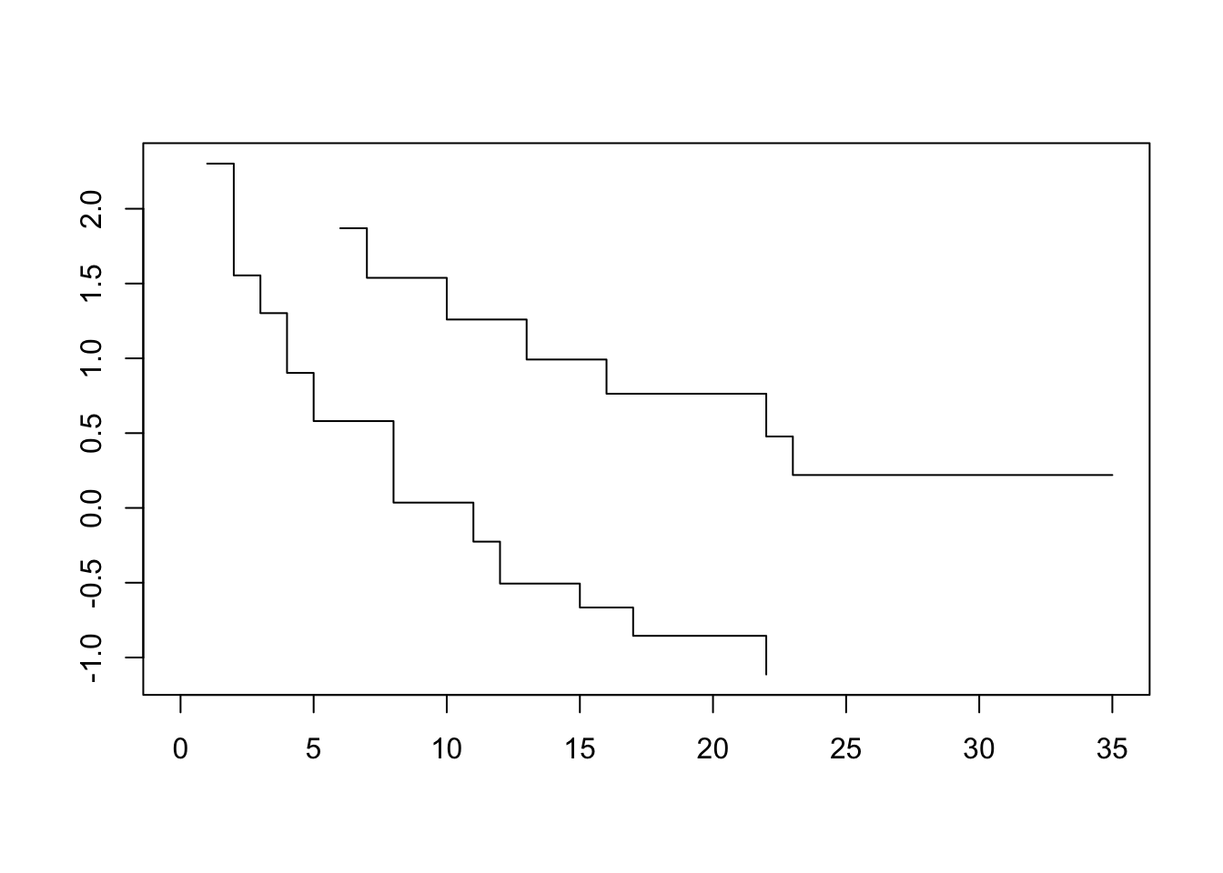

# Then consider log_wbc
plot(survfit(Surv(lifetime, death) ~ log_wbc_bin, data=lukemia), col=c("blue", "red", "black"), fun=loglog)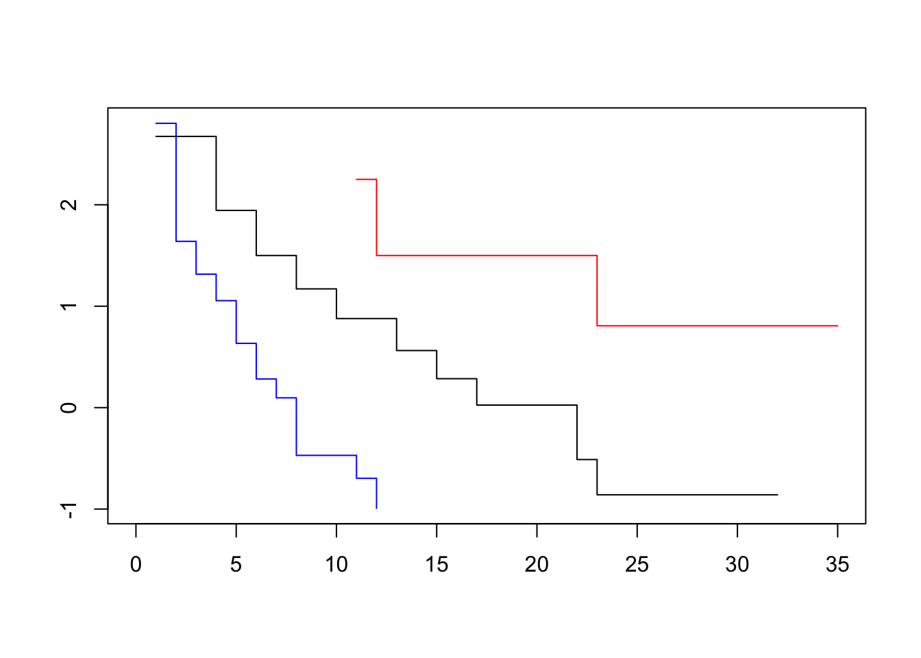

# Finally, consider sex
plot(survfit(Surv(lifetime, death) ~ sex, data=lukemia), col=c("blue", "red"), fun=loglog)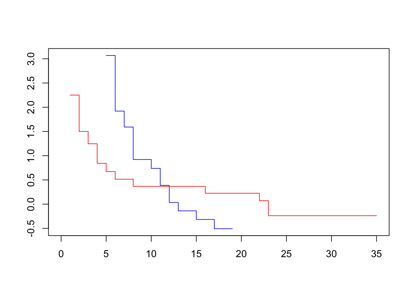

Observed versus Expected

Observed versus expected plots are the graphical equivalent of goodness-of-fit tests.

We will carry out the procedure for one variable at a time. Again, using the lukemia data, we will fit to just the treatment variable.

# Fit a cox model
fit <- coxph(Surv(lifetime, death) ~ ctl, data=lukemia)
# Construct the data frame we'd like to predict for.
df <-  data.frame(ctl = c(0, 1)) 

plot(survfit(Surv(lifetime, death) ~ ctl, data=lukemia), col=1:2)
par(new=TRUE)
plot(survfit(fit, newdata=df), lty=2, col=1:2)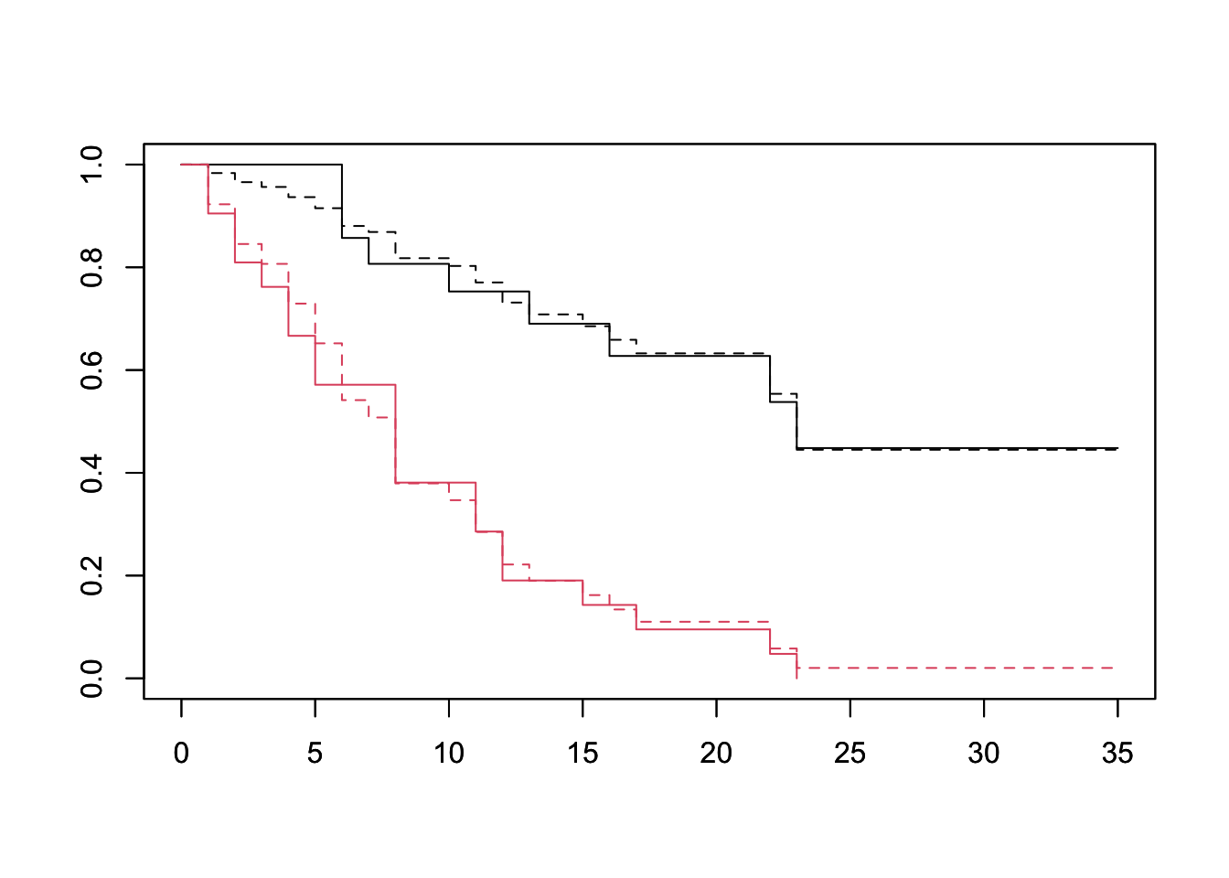

The PH assumption seems well founded when looking at the treatment variable. That is to say the treatment group’s survival is a scaling of the baseline survival of the control group.

# Fit a cox model
fit <- coxph(Surv(lifetime, death) ~ sex, data=lukemia)
# Construct the data frame we'd like to predict for.
df <-  data.frame(sex = c(0, 1)) 

plot(survfit(Surv(lifetime, death) ~ sex, data=lukemia), col=1:2)
par(new=TRUE)
plot(survfit(fit, newdata=df), lty=2, col=1:2)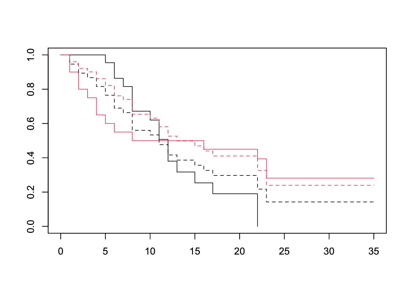

We can see a clear departure of the expected from the observed curves, especially between days 0 and 15. This suggests that sex does not conform to the PH asssumption.

Finally, we have to deal with continuous variables. There are two ways to do this: dummy coding, or using a continuous predictor.

# Fit a cox model with dummy-coding. We've already bucketed log_wbc previously.
fit <- coxph(Surv(lifetime, death) ~ log_wbc_bin, data=lukemia)
fit

## Call:
## coxph(formula = Surv(lifetime, death) ~ log_wbc_bin, data = lukemia)
## 
##                 coef exp(coef) se(coef)  z     p
## log_wbc_binlow -3.03      0.05     0.71 -4 2e-05
## log_wbc_binmed -1.46      0.23     0.45 -3 0.001
## 
## Likelihood ratio test=27  on 2 df, p=1e-06
## n= 42, number of events= 30

# Construct the data frame we'd like to predict for.
# The ordering is a bit weird because factors are constructed alphabetically in R.
df <-  data.frame(log_wbc_bin = c('high', 'low', 'med'))

plot(survfit(Surv(lifetime, death) ~ log_wbc_bin, data=lukemia), col=1:3)
par(new=TRUE)
plot(survfit(fit, newdata=df), lty=2, col=1:3)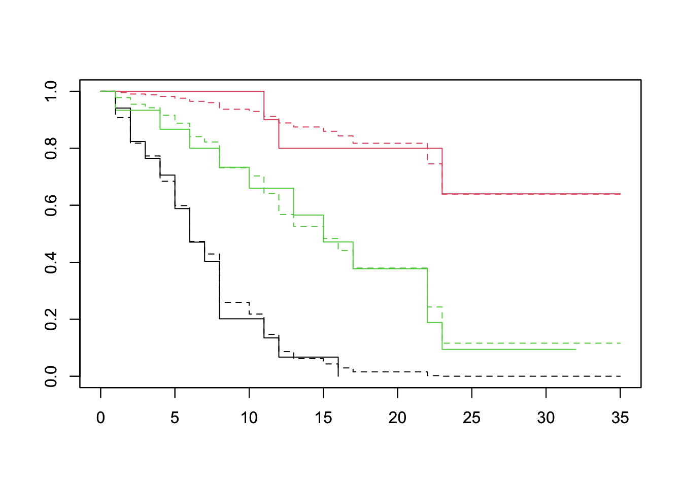

# Alternatively, we can fit log_wbc as a continuous predictor, and then predict for the means of each group.
fit <- coxph(Surv(lifetime, death) ~ log_wbc, data=lukemia)
fit

## Call:
## coxph(formula = Surv(lifetime, death) ~ log_wbc, data = lukemia)
## 
##         coef exp(coef) se(coef) z     p
## log_wbc  1.6       5.2      0.3 6 3e-08
## 
## Likelihood ratio test=35  on 1 df, p=4e-09
## n= 42, number of events= 30

# Construct the data frame we'd like to predict for.
df <- lukemia %>% group_by(log_wbc_bin) %>% summarize(log_wbc=mean(log_wbc)) %>% select(log_wbc)

## `summarise()` ungrouping output (override with `.groups` argument)

plot(survfit(Surv(lifetime, death) ~ log_wbc_bin, data=lukemia), col=1:3)
par(new=TRUE)
plot(survfit(fit, newdata=df), lty=2, col=1:3)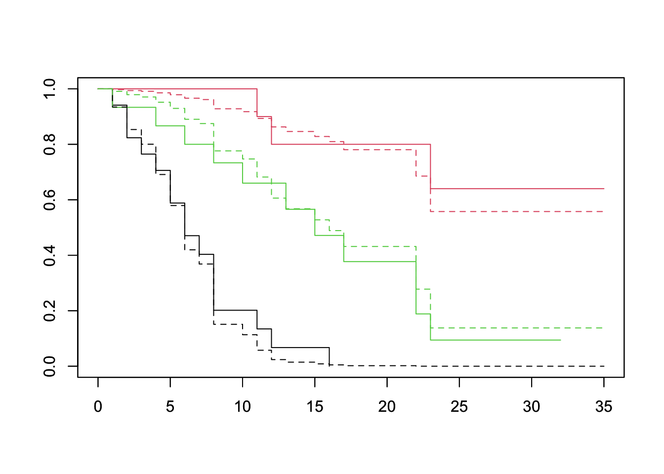

Goodness-Of-Fit Test

There are various goodness-of-fit (GOF) tests for checking Cox PH models. We will discuss the one by Harrel and Lee (1986) which adapts a test proposed by Schoenfeld (1982).

Each subject with an event will have a Schoenfeld residual per predictor. Suppose a subject i has an event at time t. Her schoenfeld residual for, say, log_wbc is her observed value of log_wbc minus a weighted average of the log_wbc values of the subjects still at risk at time t. The weights are each subject’s hazard.

If the PH assumption holds for a particular covariate, then the Schoenfeld residual is not related to survival time.

To run the test, we carry out three steps: 1. Fit the Cox PH model and obtain residuals per predictor. 2. Rank the subjects by failure time, and number then 1 through n with 1 being the earliest failure. 3. Test the correlation between 1 and 2. There should be no correlation.

fit <- coxph(Surv(lifetime, death) ~ log_wbc + ctl + sex, data=lukemia)
cox.zph(fit, transform="rank")

##          chisq df     p
## log_wbc 0.0674  1 0.795
## ctl     0.0652  1 0.798
## sex     5.5489  1 0.018
## GLOBAL  5.8647  3 0.118

We can see that we cannot reject the null for the treatment and log_wbc covariates, so there is no reason to believe they violate the PH assumption. However, sex has a p-value of 0.018, and should be taken out of the model.

Reference

• https://rpubs.com/kaz_yos/kleinbaum-ph-assumption
• Lukemia data: http://web1.sph.emory.edu/dkleinb/allDatasets/surv2datasets/anderson.dat