The Stratified Cox (SC) model allows us to control for variables that do not satisfy the proportional hazards assumption.
Instead, we estimate a separate baseline hazard per group, and then estimate the parameters jointly.
\[ h(t, X) = h_{0g}(t) exp(\sum_i^p \beta_i X_i) \] Notice the new g subscript, which indicates the stratification of units by some set of covariates.
In our previous example with leukemia patients, sex does not satisfy the PH assumption. We can stratify on sex, and give each sex their own baseline hazard.
\[ h(t, X) = h_{0s}(t) exp(\beta_{tx} X_{tx} + \beta_{logWBC} X_{logWBC}) \]
Note that since the coefficients for treatment and logWBC are shared between males and females, the estimates of hazard ratios are the same for both sexes. This feature is called the “no-interaction” assumption.
tx <- data.frame(lifetime=c(6,6,6,7,10,13,16,22,23,6,9,10,11,17,19,20,25,32,32,34,35),
                 log_wbc=c(2.31, 4.06, 3.28, 4.43, 2.96, 2.88, 3.60, 2.32, 2.57, 3.20,
                           2.80, 2.70, 2.60, 2.16, 2.05, 2.01, 1.78, 2.20, 2.53, 1.47,
                           1.45),
                 death=c(rep(TRUE,9), rep(FALSE, 12)),
                 sex_f = c(0, 1, 0, 0, 0, 0, 1, 1, 1, 0, 0, 0, 0, 0, 0, 1, 1, 1, 1, 1, 1),
                 group="tx",
                 ctl=0)
ctl <- data.frame(lifetime=c(1,1,2,2,3,4,4,5,5,8,8,8,8,11,11,12,12,15,17,22,23),
                  log_wbc=c(2.80, 5.00, 4.91, 4.48, 4.01, 4.36, 2.42, 3.49, 3.97, 3.52,
                            3.05, 2.32, 3.26, 3.49, 2.12, 1.50, 3.06, 2.30, 2.95, 2.73,
                            1.97),
                  death=c(rep(TRUE, 21)),
                  sex_f=c(1, 1, 1, 1, 1, 1, 1, 1, 0, 0, 0, 0, 1, 0, 0, 0, 0, 0, 0, 0, 1),
                  group="ctl",
                  ctl=1)
lukemia <- rbind(tx, ctl)
# We must bin log_wbc to use log-log procedure
lukemia <- lukemia %>%
  mutate(log_wbc_bin = case_when(log_wbc < 2.3 ~ 'low',
                                 log_wbc >= 2.3 & log_wbc <= 3 ~ 'med',
                                 TRUE ~ 'high'))

fit <- coxph(Surv(lifetime, death) ~ log_wbc + ctl + strata(sex_f), data=lukemia)

# Create a synthetic dataset for all the groups we want to fit.
df <- expand.grid(log_wbc=mean(lukemia$log_wbc), ctl=c(0, 1), sex_f=c(0,1)) %>% data.frame()
row.names(df) <- c("Male Tx", "Male Ctl", "Female Tx", "Female Ctl")
ggsurvplot(survfit(fit, newdata=df, data=lukemia))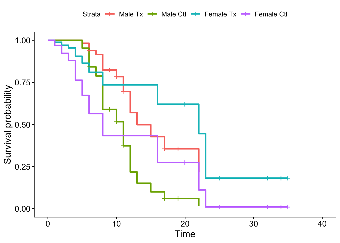
After the fit, notice that there is no coefficient associated with sex. Since the variable does not satisfy the PH assumption, its’ effect on hazard must vary with time. The likelihood for a stratified cox model is formed by taking the product across the likelihood for each stratum.
In general, if there is more than one variable we’d like to stratify on, we create a new variable with one level for each element of the cross product, and stratify on that. Numeric variables are divided into intervals.
Testing the No Interaction Assumption
When we fit a stratified sample, the model constrains the coefficients to be the same across strata. To verify that this assumption is well-founded, we can fit the models separately to the groups to see how the coefficients differ.
Let’s compare a stratified model, versus one where each strata is fit independently.
fit <- coxph(Surv(lifetime, death) ~ log_wbc + ctl + strata(sex_f), data=lukemia)
to <- tbl_regression(fit, exponentiate = TRUE)

lukemia_m <- lukemia %>% filter(sex_f == 0)
lukemia_f <- lukemia %>% filter(sex_f == 1)
fit_m <- coxph(Surv(lifetime, death) ~ log_wbc + ctl, data=lukemia_m)
fit_f <- coxph(Surv(lifetime, death) ~ log_wbc + ctl, data=lukemia_f)
tm <- tbl_regression(fit_m, exponentiate = TRUE)
tf <- tbl_regression(fit_f, exponentiate = TRUE)

tbl_merge(list(to, tm, tf), tab_spanner = c("Overall", "Male", "Female"))| Characteristic | Overall | Male | Female | ||||||
|---|---|---|---|---|---|---|---|---|---|
| HR1 | 95% CI1 | p-value | HR1 | 95% CI1 | p-value | HR1 | 95% CI1 | p-value | |
| log_wbc | 4.28 | 2.18, 8.40 | <0.001 | 3.34 | 1.25, 8.96 | 0.017 | 5.71 | 2.00, 16.3 | 0.001 |
| ctl | 2.71 | 1.07, 6.86 | 0.035 | 1.37 | 0.45, 4.12 | 0.6 | 7.23 | 1.70, 30.8 | 0.007 |
|
1
HR = Hazard Ratio, CI = Confidence Interval
|
|||||||||
We can see that for males, that the treatment does not have a statistically significant effect on the patient’s survival. On the other hand, females seem to benefit greatly from the treatment (HR 7.23).
Unfortunately, we do not have a formal way to compare our baseline model to both fit-per-sex models and come to a determination. We must reformulate our separated models into a single one in order to carry out a formal comparison:
\[ h_g(t, X) = h_{0g}(t) exp\left[ \beta_1 logWBC + \beta_2 Ctl + \beta_3 Sex * logWBC + \beta_4 Sex * Ctl \right] \] By adding interaction terms, and allowing a different baseline hazard per sex (denoted by the subscript g), we have end up fitting a separate model per sex.
For males (sex=0), the model simplifies to: \[ h_g(t, X) = h_{00}(t) exp\left[ \beta_1 logWBC + \beta_2 Ctl \right] \]
For females: \[ h_g(t, X) = h_{01}(t) exp\left[ (\beta_1 + \beta_3) logWBC + (\beta_2 + \beta_4) Ctl \right] \]
So adding the interaction terms ends up allowing each sex to be fit independently.
# Need to include strata(sex) term to indicate that we want a separate baseline hazard per sex.
fit_interaction <- coxph(Surv(lifetime, death) ~ log_wbc + ctl + log_wbc:sex_f + ctl:sex_f + strata(sex_f), data=lukemia)
ti <- tbl_regression(fit_interaction, exponentiate=TRUE)

# Let's look at all three fits next to each other
tbl_merge(list(ti, tm, tf), tab_spanner = c("Interaction", "Male", "Female"))| Characteristic | Interaction | Male | Female | ||||||
|---|---|---|---|---|---|---|---|---|---|
| HR1 | 95% CI1 | p-value | HR1 | 95% CI1 | p-value | HR1 | 95% CI1 | p-value | |
| log_wbc | 3.34 | 1.25, 8.96 | 0.017 | 3.34 | 1.25, 8.96 | 0.017 | 5.71 | 2.00, 16.3 | 0.001 |
| ctl | 1.37 | 0.45, 4.12 | 0.6 | 1.37 | 0.45, 4.12 | 0.6 | 7.23 | 1.70, 30.8 | 0.007 |
| log_wbc * sex_f | 1.71 | 0.40, 7.23 | 0.5 | ||||||
| ctl * sex_f | 5.29 | 0.86, 32.7 | 0.073 | ||||||
|
1
HR = Hazard Ratio, CI = Confidence Interval
|
|||||||||
Now that we have a model containing the interaction terms, we can test whether they are different from 0. This is because the non-interaction terms are shared, and captures the effect across sexes.
The likelihood ratio test can be used to compare the sub-model without interactions with the full model. This gives us an indication of whether the interaction terms are needed.
The likelihood ratio statistic should follow a chi-square distribution with 2 degrees of freedom, because we are testing two interaction terms.
fit_interaction <- coxph(Surv(lifetime, death) ~ log_wbc + ctl + log_wbc:sex_f + ctl:sex_f + strata(sex_f), data=lukemia)
fit_no_interaction <- coxph(Surv(lifetime, death) ~ log_wbc + ctl + strata(sex_f), data=lukemia)

l_full <- -2 * (logLik(fit_interaction)) %>% as.numeric()
l_reduced <- -2 * (logLik(fit_no_interaction)) %>% as.numeric()
print("Pvalue for likelihood ratio test is: ")
## [1] "Pvalue for likelihood ratio test is: "pchisq(l_reduced - l_full, 2, lower.tail = F)## [1] 0.1521439Our conclusion is that the interactions are not significantly different from 0, and therefore the no-interaction assumption is acceptable. This means that the coefficients can be shared between sexes.
This procedure, of creating interaction terms and running a log likelihood test, generalizes to any number of groups. We will work through an example next.
An Example with Several Stratifying Variables
# status=1 is died, 0 is censored.
# CT1 = large, CT2 = adeno, CT3 = small, CT4 = squamous
vets <- read.dta("http://web1.sph.emory.edu/dkleinb/allDatasets/surv2datasets/vets.dta")
# Code treatment as 1 for treatment, 0 for control.
vets <- vets %>% mutate(tx = tx - 1)

str(vets)
## 'data.frame': 137 obs. of 11 variables:
## $ tx : num 0 0 0 0 0 0 0 0 0 0 ...
## $ ct1 : num 0 0 0 0 0 0 0 0 0 0 ...
## $ ct2 : num 0 0 0 0 0 0 0 0 0 0 ...
## $ ct3 : num 0 0 0 0 0 0 0 0 0 0 ...
## $ ct4 : num 1 1 1 1 1 1 1 1 1 1 ...
## $ survt : num 72 411 228 126 118 10 82 110 314 100 ...
## $ perf : num 60 70 60 60 70 20 40 80 50 70 ...
## $ dd : num 7 5 3 9 11 5 10 29 18 6 ...
## $ age : num 69 64 38 63 65 49 69 68 43 70 ...
## $ priortx: num 0 10 0 10 10 0 10 0 0 0 ...
## $ status : num 1 1 1 1 1 1 1 1 1 0 ...
## - attr(*, "datalabel")= chr ""
## - attr(*, "time.stamp")= chr ""
## - attr(*, "formats")= chr [1:11] "%10.0g" "%10.0g" "%10.0g" "%10.0g" ...
## - attr(*, "types")= int [1:11] 100 100 100 100 100 100 100 100 100 100 ...
## - attr(*, "val.labels")= chr [1:11] "" "" "" "" ...
## - attr(*, "var.labels")= chr [1:11] "treatment (1=standard, 2=test)" "cell type 1 (1=large, 0=other)" "cell type 2 (1=adeno, 0=other)" "cell type 3 (1=small, 0=other)" ...
## - attr(*, "version")= int 6summary(vets)## tx ct1 ct2 ct3
## Min. :0.0000 Min. :0.0000 Min. :0.0000 Min. :0.0000
## 1st Qu.:0.0000 1st Qu.:0.0000 1st Qu.:0.0000 1st Qu.:0.0000
## Median :0.0000 Median :0.0000 Median :0.0000 Median :0.0000
## Mean :0.4964 Mean :0.1971 Mean :0.1971 Mean :0.3504
## 3rd Qu.:1.0000 3rd Qu.:0.0000 3rd Qu.:0.0000 3rd Qu.:1.0000
## Max. :1.0000 Max. :1.0000 Max. :1.0000 Max. :1.0000
## ct4 survt perf dd
## Min. :0.0000 Min. : 1.0 Min. :10.00 Min. : 1.000
## 1st Qu.:0.0000 1st Qu.: 25.0 1st Qu.:40.00 1st Qu.: 3.000
## Median :0.0000 Median : 80.0 Median :60.00 Median : 5.000
## Mean :0.2555 Mean :121.6 Mean :58.57 Mean : 8.774
## 3rd Qu.:1.0000 3rd Qu.:144.0 3rd Qu.:75.00 3rd Qu.:11.000
## Max. :1.0000 Max. :999.0 Max. :99.00 Max. :87.000
## age priortx status
## Min. :34.00 Min. : 0.00 Min. :0.0000
## 1st Qu.:51.00 1st Qu.: 0.00 1st Qu.:1.0000
## Median :62.00 Median : 0.00 Median :1.0000
## Mean :58.31 Mean : 2.92 Mean :0.9343
## 3rd Qu.:66.00 3rd Qu.:10.00 3rd Qu.:1.0000
## Max. :81.00 Max. :10.00 Max. :1.0000Let’s fit a Cox PH model and test whether all covariates meet the PH assumption.
fit <- coxph(Surv(survt, status) ~ tx + ct1 + ct2 + ct3 + perf + age + priortx + dd, data=vets)
summary(fit)
## Call:
## coxph(formula = Surv(survt, status) ~ tx + ct1 + ct2 + ct3 +
## perf + age + priortx + dd, data = vets)
##
## n= 137, number of events= 128
##
## coef exp(coef) se(coef) z Pr(>|z|)
## tx 2.946e-01 1.343e+00 2.075e-01 1.419 0.15577
## ct1 4.013e-01 1.494e+00 2.827e-01 1.420 0.15574
## ct2 1.196e+00 3.307e+00 3.009e-01 3.975 7.05e-05 ***
## ct3 8.616e-01 2.367e+00 2.753e-01 3.130 0.00175 **
## perf -3.282e-02 9.677e-01 5.508e-03 -5.958 2.55e-09 ***
## age -8.706e-03 9.913e-01 9.300e-03 -0.936 0.34920
## priortx 7.159e-03 1.007e+00 2.323e-02 0.308 0.75794
## dd 8.132e-05 1.000e+00 9.136e-03 0.009 0.99290
## ---
## Signif. codes: 0 '***' 0.001 '**' 0.01 '*' 0.05 '.' 0.1 ' ' 1
##
## exp(coef) exp(-coef) lower .95 upper .95
## tx 1.3426 0.7448 0.8939 2.0166
## ct1 1.4938 0.6695 0.8583 2.5996
## ct2 3.3071 0.3024 1.8336 5.9647
## ct3 2.3669 0.4225 1.3799 4.0597
## perf 0.9677 1.0334 0.9573 0.9782
## age 0.9913 1.0087 0.9734 1.0096
## priortx 1.0072 0.9929 0.9624 1.0541
## dd 1.0001 0.9999 0.9823 1.0182
##
## Concordance= 0.736 (se = 0.021 )
## Likelihood ratio test= 62.1 on 8 df, p=2e-10
## Wald test = 62.37 on 8 df, p=2e-10
## Score (logrank) test = 66.74 on 8 df, p=2e-11# Check for PH assumption
cox.zph(fit)## chisq df p
## tx 0.2644 1 0.60712
## ct1 5.5033 1 0.01898
## ct2 6.7929 1 0.00915
## ct3 3.9879 1 0.04583
## perf 12.9352 1 0.00032
## age 1.8288 1 0.17627
## priortx 2.1656 1 0.14113
## dd 0.0129 1 0.90961
## GLOBAL 34.5525 8 3.2e-05Our test reveals that cell-type, and performance do not meet the PH assumption. We will use stratification to pull these two covariates out of the model. Cell type is already a categorical variable, but perf is a integer that runs from 0 for worst to 100 for best. We will divide perf into two groups using the median, 60, as the cut point. Stratifying by all possible combinations gives us 8 groups total.
vets <- vets %>%
  mutate(perf_category = case_when(perf >= 60 ~ 1, TRUE ~ 0))

# We will form the groups by pasting together the variables, and then massaging it into a factor.
vets_stratified <- vets %>%
  mutate(ct_perf=paste0(ct1, ct2, ct3, perf_category)) %>%
  select(tx, age, ct_perf, status, survt)

fit <- coxph(Surv(survt, status) ~ tx + age + strata(ct_perf), data=vets_stratified)
summary(fit)
## Call:
## coxph(formula = Surv(survt, status) ~ tx + age + strata(ct_perf),
## data = vets_stratified)
##
## n= 137, number of events= 128
##
## coef exp(coef) se(coef) z Pr(>|z|)
## tx 0.12779 1.13631 0.20854 0.613 0.54
## age -0.00127 0.99873 0.01011 -0.126 0.90
##
## exp(coef) exp(-coef) lower .95 upper .95
## tx 1.1363 0.880 0.7551 1.710
## age 0.9987 1.001 0.9791 1.019
##
## Concordance= 0.518 (se = 0.04 )
## Likelihood ratio test= 0.38 on 2 df, p=0.8
## Wald test = 0.38 on 2 df, p=0.8
## Score (logrank) test = 0.38 on 2 df, p=0.8Our stratified model shows that neither treatment, nor age have an effect on survival.
# Here is the no-interaction model again
fit_reduced <- coxph(Surv(survt, status) ~ tx + age + strata(ct_perf), data=vets_stratified)
fit_full <- coxph(Surv(survt, status) ~ tx + age + tx:ct_perf + age:ct_perf + strata(ct_perf), data=vets_stratified)
summary(fit_full)
## Call:
## coxph(formula = Surv(survt, status) ~ tx + age + tx:ct_perf +
## age:ct_perf + strata(ct_perf), data = vets_stratified)
##
## n= 137, number of events= 128
##
## coef exp(coef) se(coef) z Pr(>|z|)
## tx 0.304398 1.355808 0.664669 0.458 0.647
## age -0.001577 0.998424 0.030104 -0.052 0.958
## tx:ct_perf0001 -1.051842 0.349294 0.868262 -1.211 0.226
## tx:ct_perf0010 0.568051 1.764825 0.855773 0.664 0.507
## tx:ct_perf0011 0.010718 1.010776 0.822590 0.013 0.990
## tx:ct_perf0100 -1.191997 0.303614 0.956623 -1.246 0.213
## tx:ct_perf0101 0.575167 1.777427 0.972588 0.591 0.554
## tx:ct_perf1000 2.332395 10.302588 1.772412 1.316 0.188
## tx:ct_perf1001 0.504738 1.656551 0.954146 0.529 0.597
## age:ct_perf0001 0.052155 1.053539 0.048349 1.079 0.281
## age:ct_perf0010 -0.058974 0.942731 0.042265 -1.395 0.163
## age:ct_perf0011 0.035731 1.036377 0.038292 0.933 0.351
## age:ct_perf0100 -0.046228 0.954824 0.045178 -1.023 0.306
## age:ct_perf0101 -0.039624 0.961150 0.045020 -0.880 0.379
## age:ct_perf1000 0.078653 1.081828 0.064003 1.229 0.219
## age:ct_perf1001 -0.036529 0.964130 0.045941 -0.795 0.427
##
## exp(coef) exp(-coef) lower .95 upper .95
## tx 1.3558 0.73757 0.36849 4.988
## age 0.9984 1.00158 0.94122 1.059
## tx:ct_perf0001 0.3493 2.86292 0.06370 1.915
## tx:ct_perf0010 1.7648 0.56663 0.32981 9.444
## tx:ct_perf0011 1.0108 0.98934 0.20159 5.068
## tx:ct_perf0100 0.3036 3.29365 0.04656 1.980
## tx:ct_perf0101 1.7774 0.56261 0.26419 11.958
## tx:ct_perf1000 10.3026 0.09706 0.31935 332.374
## tx:ct_perf1001 1.6566 0.60366 0.25529 10.749
## age:ct_perf0001 1.0535 0.94918 0.95829 1.158
## age:ct_perf0010 0.9427 1.06075 0.86778 1.024
## age:ct_perf0011 1.0364 0.96490 0.96144 1.117
## age:ct_perf0100 0.9548 1.04731 0.87391 1.043
## age:ct_perf0101 0.9612 1.04042 0.87997 1.050
## age:ct_perf1000 1.0818 0.92436 0.95429 1.226
## age:ct_perf1001 0.9641 1.03720 0.88111 1.055
##
## Concordance= 0.627 (se = 0.035 )
## Likelihood ratio test= 24.77 on 16 df, p=0.07
## Wald test = 23.03 on 16 df, p=0.1
## Score (logrank) test = 25.07 on 16 df, p=0.07l_full <- -2 * (logLik(fit_full)) %>% as.numeric()
l_reduced <- -2 * (logLik(fit_reduced)) %>% as.numeric()
print("Pvalue for likelihood ratio test is: ")## [1] "Pvalue for likelihood ratio test is: "# 14 additional coefficients in the full model, so df=14
pchisq(l_reduced - l_full, 14, lower.tail = F)## [1] 0.04102486Seems like the LRT is significant, rejecting the null (reduced model is sufficient), and therefore we would continue with the full model.