Formulation of Extended Cox Model

We can write a time-dependent Cox model as follows:

\[ h(t, X(t)) = h_0(t) * exp \left[ \sum_i \beta_i X_i + \sum_j \delta_j X_j(t) \right] \]

As with the simpler Cox PH model, the coefficients are estimated using a maximum likelihood procedure. However, the computations are more complicated because the risk sets must account for the time dependent variables.

Importantly, the extended cox model assumes that the effect of the time-dependent variable on the survival probability at time t depends on the value of this variable at that same time t, and not on the value at any earlier or later time.

We can modify the model by incorporating lag-time variables. For example, if we are looking at employment status on week t, then only that would affect the hazard. However, to allow for, say, a one-week lag, the employment status variable may be modified so that the hazard model at time t looks at employment status at time t-1.

Hazard Ratio for Extended Cox Models

The hazard ratio is now a function of time and the proportional hazards assumption no longer holds.

\[ \begin{align} HR(t) &= \frac{h(t, X^*(t))}{h(t, X(t))} \\ & = exp \left[ \sum_i \beta_i (X^*_i - X_i) + \sum_j \delta_j (X^*_j(t) - X_j(t)) \right] \end{align} \] Here is a simple example. Suppose that there is only one time-independent predictor, namely exposure (0/1), and one time-dependent defined variable exposure*time. Let’s take a look at the form of the model:

\[ h(t, X(t)) = h_0(t) exp \left[ \beta E + \delta E * t \right] \]

Take the ratio of two individuals X, and X* with exposures 0 and 1 respectively, we get:

\[ \begin{align} HR(t) &= \frac{h(t, E=1)}{h(t, E=0)} \\ &= exp(\beta(1 - 0) + \delta (1 * t - 0*t)) \\ &= exp(\beta+ \delta t) \end{align} \]

We can see that an exposed individual has a hazard ratio that is proportional to beta, and this ratio goes up over time in proportion to delta.

Note that delta itself is not time dependent, meaning that the risk is changed by delta no matter where this change occurs.

As another example, let’s consider a factory where there is a measure for chemical exposure by week. Each individual can have a different exposure “signature”. For example, 10011 means that the individual was exposed for the first, fourth and fifth weeks.

The model would be \[ h(t, X(t)) = h_0(t) exp \left[ \delta E(t) \right] \]

Using the extended cox model to assess time independent variables for PH assumption

Say we want to define the Cox PH model as follows: \[ h(t, X) = h_0(t) exp \left[ \sum_i \beta_i X_i \right] \]

To assess whether each variable satisfies the PH assumption, we extend the model with a product term of each covariate with a function of time, g(t).

\[ h(t, X) = h_0(t) exp \left[ \sum_i \beta_i X_i + \delta_i X_i g(t) \right] \]

We would just use the LRT test to test whether the PH assumption (null hypothesis) holds, or if the time dependence is required.

Example - Treatment of Heroin Addiction

In a 1991 Australian study, Caplehorn et al. studied the retention of heroin addicts in two different methadone clinics. The survival time, T, was measured in days until a patient dropped out or was censored at the end of the study. The two clinics differed in their overall treatment plan.

addicts <- read.dta("http://web1.sph.emory.edu/dkleinb/allDatasets/surv2datasets/addicts.dta")

str(addicts)

## 'data.frame':    238 obs. of  6 variables:
##  $ id    : num  1 2 3 4 5 6 7 8 9 10 ...
##  $ clinic: num  1 1 1 1 1 1 1 1 1 1 ...
##  $ status: num  1 1 1 1 1 1 1 0 1 1 ...
##  $ survt : num  428 275 262 183 259 714 438 796 892 393 ...
##  $ prison: num  0 1 0 0 1 0 1 1 0 1 ...
##  $ dose  : num  50 55 55 30 65 55 65 60 50 65 ...
##  - attr(*, "datalabel")= chr ""
##  - attr(*, "time.stamp")= chr ""
##  - attr(*, "formats")= chr [1:6] "%10.0g" "%10.0g" "%10.0g" "%10.0g" ...
##  - attr(*, "types")= int [1:6] 100 100 100 100 100 100
##  - attr(*, "val.labels")= chr [1:6] "" "" "" "" ...
##  - attr(*, "var.labels")= chr [1:6] "Subject ID" "Coded 1 or 2" "status (0=censored, 1=endpoint)" "survival time in days" ...
##  - attr(*, "version")= int 6

Column Definitions:

• status: 0 = censored, 1 = departed / failed
• prison: 0 = none, 1 = any
• dose: maximum methadone dose (mg / day)

The major exposure variable was clinic, with prison and maximum methadone dose as control variables.

Starting with the simplest model, we will fit a Cox PH model to clinic, dose, and prison status.

fit <- coxph(Surv(survt, status) ~ clinic + prison + dose, data=addicts)
summary(fit)

## Call:
## coxph(formula = Surv(survt, status) ~ clinic + prison + dose, 
##     data = addicts)
## 
##   n= 238, number of events= 150 
## 
##             coef exp(coef)  se(coef)      z Pr(>|z|)    
## clinic -1.009896  0.364257  0.214889 -4.700 2.61e-06 ***
## prison  0.326555  1.386184  0.167225  1.953   0.0508 .  
## dose   -0.035369  0.965249  0.006379 -5.545 2.94e-08 ***
## ---
## Signif. codes:  0 '***' 0.001 '**' 0.01 '*' 0.05 '.' 0.1 ' ' 1
## 
##        exp(coef) exp(-coef) lower .95 upper .95
## clinic    0.3643     2.7453    0.2391    0.5550
## prison    1.3862     0.7214    0.9988    1.9238
## dose      0.9652     1.0360    0.9533    0.9774
## 
## Concordance= 0.665  (se = 0.025 )
## Likelihood ratio test= 64.56  on 3 df,   p=6e-14
## Wald test            = 54.12  on 3 df,   p=1e-11
## Score (logrank) test = 56.32  on 3 df,   p=4e-12

# Test for PH assumption
cox.zph(fit)

##         chisq df       p
## clinic 11.159  1 0.00084
## prison  0.839  1 0.35969
## dose    0.515  1 0.47310
## GLOBAL 12.287  3 0.00646

We can see that clinic does not satisfy the PH assumption. The other two variables, prison and dose, are not significant suggesting that we can keep it in the PH portion of the model.

Let’s take a closer look at clinic.

# Stratify by clinic to give each their own baseline hazard
fit <- coxph(Surv(survt, status) ~ strata(clinic) + prison + dose, data=addicts)
ggadjustedcurves(fit) + geom_vline(xintercept = 365)

## Warning in .get_data(fit, data): The `data` argument is not provided. Data will
## be extracted from model fit.

## The variable argument is missing. Using clinic as extracted from strata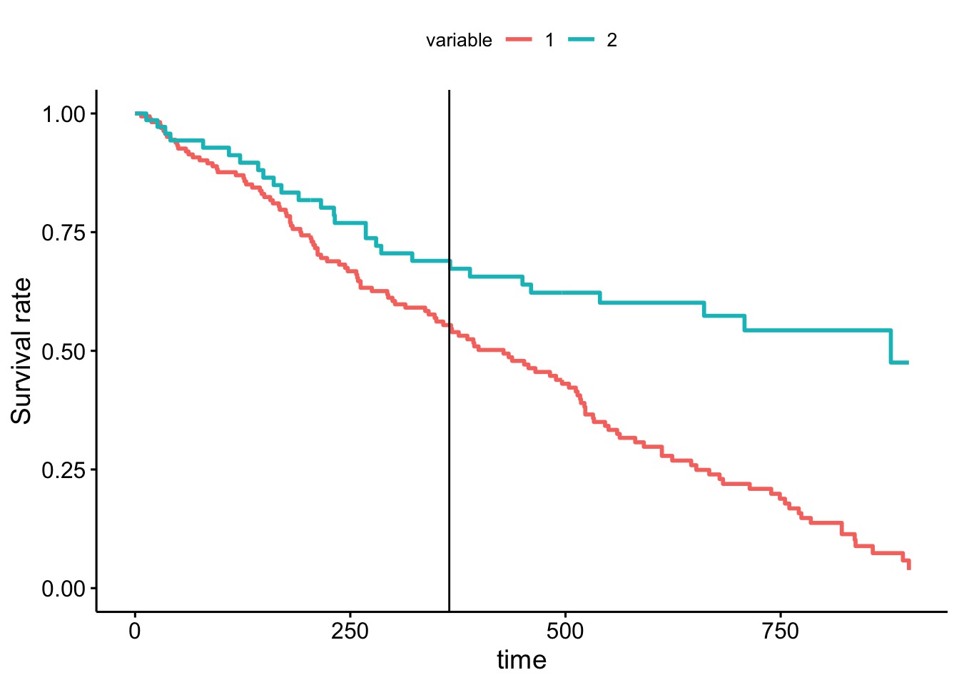

Clearly, the survival curves of the two clinics are not proportional to each other. Stratifying by clinic, we observe that the clinics perform similarly up to a year, before markedly diverging. We can conclude that clinic 2 is much better at retaining their patients.

We’d like to capture the idea that the curves diverge markedly after a year. To do so, we create a function that is 0 when \(t < 365\), and 1 when \(t \geq 365\). This is called a heaviside function. Adding it to the model gives us the HR before and after the cut.

\[ h(t, X(t)) = h_0(t) * exp \left[ \beta_1 clinic + \beta_2 dose + \beta_3 prison + \delta * clinic * g(t) \right] \]

Then for an individual in different clinics, but before 365, we would have a HR of \(exp(\beta_1)\). And for individuals who are in different clinics, and after 365, we would have HR \(exp(\beta_1 + \delta)\)

Alternatively, we could formulate this as a coefficient on indicators for before/after the cut. These two different deltas would represent the effect of clinic. \[ h(t, X(t)) = h_0(t) * exp \left[ \beta_2 dose + \beta_3 prison + \delta_1 * clinic * g_1(t) + \delta_2 * clinic * g_2(t) \right] \]

# Transform addicts data into counting process
head(addicts)

##   id clinic status survt prison dose
## 1  1      1      1   428      0   50
## 2  2      1      1   275      1   55
## 3  3      1      1   262      0   55
## 4  4      1      1   183      0   30
## 5  5      1      1   259      1   65
## 6  6      1      1   714      0   55

# Start with all columns except time, then merge in the failure event.
addicts.cp <- tmerge(
  addicts %>% select(id, clinic, prison, dose),
  addicts %>% select(id, survt, status),
  id=id,
  failure=event(survt, status))
addicts.cp <- tmerge(
  addicts.cp,
  addicts %>% mutate(time_365=365),
  id=id,
  after_365 = tdc(time_365))
# Add a before365 variable
addicts.cp <- addicts.cp %>% 
  mutate(tx= ifelse(clinic == 1, 1, 0),
    before_365 = 1 - after_365)

extended_fit <- coxph(
  Surv(tstart, tstop, failure) ~ dose + prison + tx:before_365 + tx:after_365,
  data=addicts.cp)
summary(extended_fit)

## Call:
## coxph(formula = Surv(tstart, tstop, failure) ~ dose + prison + 
##     tx:before_365 + tx:after_365, data = addicts.cp)
## 
##   n= 360, number of events= 150 
## 
##                    coef exp(coef)  se(coef)      z Pr(>|z|)    
## dose          -0.035480  0.965142  0.006435 -5.514 3.52e-08 ***
## prison         0.377951  1.459291  0.168415  2.244   0.0248 *  
## tx:before_365  0.459373  1.583081  0.255290  1.799   0.0720 .  
## tx:after_365   1.830517  6.237113  0.385954  4.743 2.11e-06 ***
## ---
## Signif. codes:  0 '***' 0.001 '**' 0.01 '*' 0.05 '.' 0.1 ' ' 1
## 
##               exp(coef) exp(-coef) lower .95 upper .95
## dose             0.9651     1.0361    0.9530    0.9774
## prison           1.4593     0.6853    1.0490    2.0300
## tx:before_365    1.5831     0.6317    0.9598    2.6110
## tx:after_365     6.2371     0.1603    2.9272   13.2895
## 
## Concordance= 0.68  (se = 0.023 )
## Likelihood ratio test= 74.25  on 4 df,   p=3e-15
## Wald test            = 57.48  on 4 df,   p=1e-11
## Score (logrank) test = 64.22  on 4 df,   p=4e-13

We can see that after 365, the choice of clinic really matters with a hazard ratio of 6.23.

Dividing the time period into two is quite coarse. In our initial plot, we observed that the gap survival curves continues to increase over time. Let’s model that directly.

addicts.cp <- survSplit(addicts, cut=addicts$survt[addicts$status==1],
                        end="survt", event="status", start="start")
addicts.cp <- addicts.cp %>% mutate(tx = ifelse(clinic == 1, 1, 0))
direct_interaction_fit <- coxph(Surv(start, survt, status) ~ dose + prison + tx + tx:survt, data=addicts.cp)

## Warning in coxph(Surv(start, survt, status) ~ dose + prison + tx + tx:survt, : a
## variable appears on both the left and right sides of the formula

summary(direct_interaction_fit)

## Call:
## coxph(formula = Surv(start, survt, status) ~ dose + prison + 
##     tx + tx:survt, data = addicts.cp)
## 
##   n= 18708, number of events= 150 
## 
##                coef  exp(coef)   se(coef)      z Pr(>|z|)    
## dose     -0.0351865  0.9654253  0.0064425 -5.462 4.72e-08 ***
## prison    0.3899661  1.4769307  0.1688856  2.309   0.0209 *  
## tx       -0.0193951  0.9807918  0.3471700 -0.056   0.9554    
## tx:survt  0.0030207  1.0030253  0.0009453  3.195   0.0014 ** 
## ---
## Signif. codes:  0 '***' 0.001 '**' 0.01 '*' 0.05 '.' 0.1 ' ' 1
## 
##          exp(coef) exp(-coef) lower .95 upper .95
## dose        0.9654     1.0358    0.9533    0.9777
## prison      1.4769     0.6771    1.0607    2.0564
## tx          0.9808     1.0196    0.4967    1.9368
## tx:survt    1.0030     0.9970    1.0012    1.0049
## 
## Concordance= 0.682  (se = 0.023 )
## Likelihood ratio test= 76.13  on 4 df,   p=1e-15
## Wald test            = 57.76  on 4 df,   p=9e-12
## Score (logrank) test = 67.09  on 4 df,   p=9e-14

See Kleinberg and Klein (p264) for calculation of confidence intervals.